Mission Juno -- Waves Investigation

Experiment Data Record (EDR) Format

Version 1 -- 2014-05-17

Prepared by

C. W. Piker

Dept. of Physics & Astronomy
The University of Iowa
Iowa City, IA 52242

This document has been reviewed for export control and does NOT contain technical information controlled under the International Traffic in Arms Regulations (22 CFR 120-130).

Contents
1. Overview
    1.1 Common Properties
    1.2 On-Board Manipulations
    1.3 Output to Spacecraft verses Level 2 Packets
    1.4 Extra Processing for Downmixed Waveforms

2. WGDS Packet Envelope
    2.1 Prefix Record
    2.2 Header Blocks
    2.3 Data (Payload) Blocks
    2.4 CRC-CCITT Algorithm

3. Science Data Packets
    3.1 Sample Vector Types (The PSID)
    3.2 Science Data Status Header Block
    3.3 Other Header Blocks
    3.4 Data Section
    3.5 Process for Converting from L2 to L3 data

4. Housekeeping Packets
    4.1 Sub-second Collect Time Adjustments
    4.2 Micro-packets

1. Overview: From Measurements to CODMAC Level 2 Files

The Level 2 volume, JNOWAV_0000 exists to "safe" low level binary Waves EDRs (Experiment Data Records) and Housekeeping packets. These data are not intended for general use. The Level 3 volume, JNOWAV_1000, provides calibrated, fixed-length records which should be used if at all possible for the task at hand. Persons wishing to process Level 2 records anyway should (in addition to reading this document) contact the Waves instrument team before proceeding.

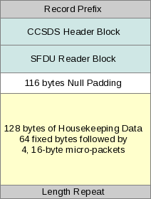
Waves science EDRs are not fixed length and thus cannot be specified via standard PDS labels. Because of this limitation, Waves EDR records are detailed in this document. Waves housekeeping records contain both a fixed format 64 byte section followed by 4, variable content, 16 byte records. The fixed section of the Waves housekeeping packets are fully defined via PDS labels, while the variable content section is briefly touched on in Section 4 below.

Prerequisite: This document delves into some of the details of handling low-level Waves instrument data. The VOLSIS.HTM document on this volume provides a higher-level overview of the Juno Mission, the Waves Instrument and it's data products. Before reading this document readers should first be familiar with Section 1.6, all of Section 2, and Appendix C of VOLSIS.HTM before proceeding.

1.1 Common Properties

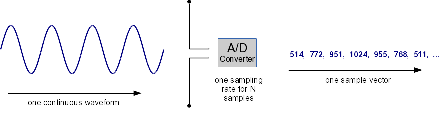
Waves measurements begin as digital conversions of analog voltage states. In this document, a set of conversion values which are,

• taken from a single A/D device,
• from the output of a single sensor,
• at constant pre-amp and receiver gain settings,
• and sampled at a uniform time spacing smaller than the low frequency cutoff period,

Inside the Waves instrument most sample vectors initially represent a voltage wave in time. If the voltage wave was driven by the electric antenna then it's an electric sample vector, if it was driven by the magnetic sensor then it's a magnetic sample vector.

Figure 1.1: Origin of most Waves data values

Raw sample vectors can be transmitted to the Juno spacecraft for later delivery to the ground. This mode of operation is called Burst Mode. Typically though, the time ordered sample vector is converted to a frequency ordered sample vector via the instrument's on-board Fourier Transform hardware. The transformed vector is further reduced via simple averaging into frequency bins. Sending reduced frequency vectors saves quite a bit of space while still providing a good overview of the instrument's environment. This mode of operation is call Survey Mode. No mater the transformations applied to the sample vector it still retains it's identity and has associated with it the following fixed properties:

• Start Time - When was sampling initiated
• Sample Frequency - How fast were measurements taken
• Initial length - How many measurements were taken
• Analog Hardware State - What was the configuration of the upstream analog hardware when the measurements were taken

1.2 On-board Manipulations

Sample vectors may under go one or more of the following operations on-board before being delivered to the Juno spacecraft data systems:

1. Conversion from time domain to frequency domain
2. Averaging in the frequency domain
3. Lossy compression by conversion to 9-bit floats
4. Loss-less compression using the Rice compression algorithm
5. Segmentation into smaller sample vectors

On-board manipulations two and three (averaging over frequency and 9-bit conversion) introduce permanent changes to the data. The first operation (conversion to the frequency domain) is only done on-board in preparation for frequency averaging so the fact that it is a reversible change is irrelevant. The last two operations (Rice compression and segmentation) are reversed before Level 2 data files are written to the JNOWAV_0000 volume. No matter the on-board operations preformed on a sample vector it still maintains it's identity. The vector's start time, sample frequency, initial length and analog state properties are retained and passed down, in some form, with the data values themselves.

1.3 Output to Spacecraft verses Level 2 Packets

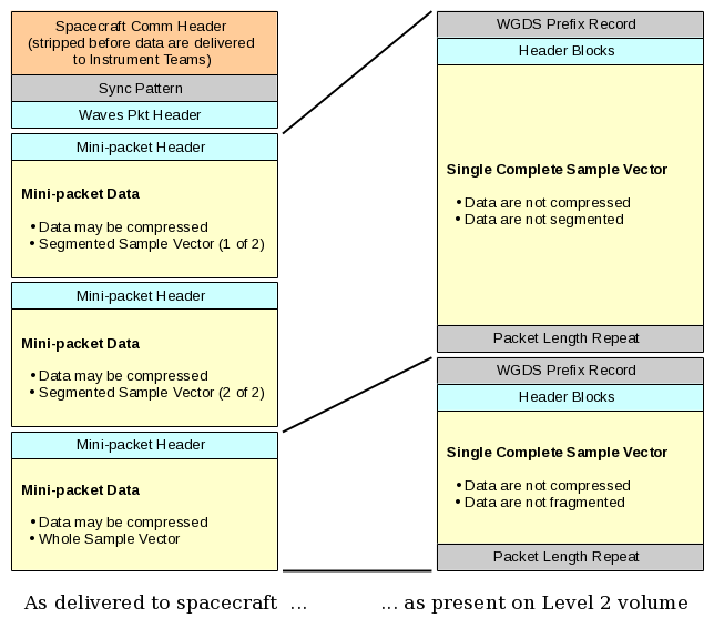
Figure 1.2: Pre-Level 2 Processing

In order to transmit information in an orderly way from Waves to Juno some sort of structure needs to be defined. Inside Waves, all sample vectors are organized into Waves Mini-Packets, which are then grouped into Waves Packets before transmission out to the spacecraft. This organization is represented in the left-hand structure in Figure 1.2.

Ideally one mini-packet would contain one sample vector. The header portion of the packet would provide the essential properties, Start Time, Sensor Selection, Gain States, Sampling Rate or Frequency Bins, Vector length and Digital Resolution. However this would make a very large header and since the Waves instrument only generates a small handful of different types of sample vectors, much of this information is provided in external look-up tables. The mini-packet headers themselves only carry a look-up table ID which must be used to determine many of the properties.

Also, it would be nice if one mini-packet always contained an entire sample vector, however some of the vectors generated by Waves are too large to fit in a single transmission unit to the spacecraft, and thus must be segmented into multiple units. These fragments each receive their own mini-packet header. Inside the header is a segment number which is used by ground software to re-assemble whole sample vectors.

In addition to these complications Waves also compresses data via two different schemes, (1) Rice Compression, which is loss-less and is used to compress the high resolution WAVES_BURST products, and (2) 9-bit float conversion which is lossy and is used to reduce the size of WAVES_SURVEY products.

Before data are written to the JNOWAV_0000 volume, the following operations are preformed:

• Unpack: Individual mini-packets are encapsulated into individual Waves Ground Data System (WGDS) packets.
  
  
• Unsegment: WGDS packets containing segments of single sample vectors are combined WGDS packets containing whole sample vectors.
  
  
• Decompress: Compressed data sections in WGDS packets are decompressed.
  
  
• Side-band Recovery: WGDS packets containing sets of downmixed data from Waves High Frequency Receivers are resolved into spectra (explained below).

1.4 Extra Processing for Downmixed Waveforms

The Waves high-frequency receivers are able to record high-resolution frequency information for signals that occur far above their sampling frequency of 1.3125 MHz using frequency down-mixing. Why this works is covered in Appendix C of the VOLSIS.HTM document. In addition to unsegmenting and decompressing Waves mini-packets. Ground software also combines HFR in-phase (I) and quadrature (Q) waveforms into a frequency spectrum centered on the mixer frequency and extending to plus and minus the Nyquist frequency of the down-linked waveforms. Like all level 2 data, the resulting spectrum is not calibrated but is still in units of data-numbers. The algorithm for doing this follows:

• Find matching sets I and Q waveform packets in the as-delivered data product files.
• Generate a complex number by placing all the Q waveform values in the real part and all the I waveform values in the imaginary part. (Q and I are labeled backwards, hence the odd convention)
• Apply a Hann window to the complex waveform.
• Run an DFT from -N/2 to N/2 - 1, normalize as required by the algorithm's instructions.
• Most FFT algorithm's provide values from 0 to N, for those the upper-half range must be shifted down by N.

It should be evident by now that quite a bit of processing is required to produce the just the Level 2 files. So, this document does not provide sufficient to information to process raw Waves science data products off the spacecraft up to useful calibrated products. The assumption then is that one has Level 2 products, by some means, and wishes to produce calibrated Level 3 files.

2. WGDS Packet Envelope

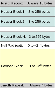
Figure 2.1: WGDS Packet Format

The basic unit of data generated by Waves and delivered to the Juno spacecraft C&DH system is called an mini-packet. Waves mini-packets are formatted to meet restrictions on instrument-to-spacecraft packet lengths and to efficiently utilize the available telemetry bandwidth. To save space, Waves Level 2 data makes copious use of bit fields, employs loss-less compressed, and truncates SCLKs. C&DH Packet length limitations require Waves to segment long sample vectors across multiple mini-packets. All this complicated in-flight packaging must be undone on the ground to recover the collected waveforms and spectra.

To provide room for ancillary data and large measurements each as-delivered, mini-packet is embedded inside a WGDS (Waves Ground Data System) packet upon receipt by the Waves instrument team. Both science and housekeeping data are placed in WGDS wrappers. All WGDS packets consist of:

• A 16-byte prefix, which contains the data and header lengths

• 1-N header blocks to record ancillary information

• A data block

• The packet length repeated

It is possible for a generic algorithm to navigate L2 data files without understanding the details of each header and data section.

Figure 2.1 provides the general structure of the ground processing packets. On the JNOWAV_0000 volume, all .DAT (housekeeping) and .PKT (science records) files are composed of a stream of these packets and only these packets. There are no other headers or footers in the files.

2.1 Prefix Record

Note: In this document all base 16 numbers are prefixed with the characters '0x', as this is standard in most common programming languages.

There is one prefix per WGDS packet, it is always 16 bytes long. The first 4 bytes are the sync pattern 0xFA, 0x6C, 0x27, 0x41. This is useful in the case that a file becomes fragmented or has invalid length information for one or more packets. Table 2.1 defines the prefix bytes in ascending address order.

WGDS Packet prefix field definitions:

CRC: A unsigned 16-bit MSB (Most Significant Byte) first integer containing the CRC-CCITT of everything that follows for this packet up to and including the trailing length bytes. See Section 1.4 for a definition of the CRC-CCITT algorithm in the C language.

Non-Data Length: An unsigned 16-bit MSB first integer containing the number of bytes in the WGDS headers alone, this includes the entire 4-byte sync pattern and the trailing 4 length bytes. Waves packets always pad the headers out to 256 bytes. This combined with the 4 trailing length bytes means that the non-data length will always be at least 260.

Total Packet Length: An unsigned 32-bit MSB first integer containing the number of bytes in the total packet, including all data, all headers, all padding and the trailer bytes.

NAIF ID: The NAIF SPICE ID for Juno, this is always -61, or 0xFF 0xC3 as hex bytes. Note that the NAIF ID sets the name space or "code table" for the header block IDs, programs IDs and the content indicator byte below.

Content Indicator Byte: An identifier for the contents of the packet. For Waves this byte consists of two parts, the upper 4 bits are the Data Kind Indicator and may have one of the following values:

• 0x6 -- Down-link data (Waves housekeeping)

• 0x8 -- Science Data

The lower bits are the Data Contents Indicator. This value denotes how many processing stages have been applied to the data contents. Upon receipt by the Waves IOT it will have the value 0x1, by the time science packets are ready for delivery to the PDS the value will be 0x5. A list of all values follows:

• 0x1 - Raw IDP (Waves housekeeping stops at this processing level)

• 0x2 through 0x4 -- See DOCUMENT/WAVESEDR/WAVESBLKS.TXT

• 0x5 - 1 Measurement (Waves science data stops at this processing level)

2.2 Header Blocks

The rest of the header is series of Header Blocks, each of which may be up to 256 bytes in size and always starts with a size byte and a block ID byte. At a minimum, this provides sufficient information for programs to skip over blocks that are unrecognized. To reiterate, all WGDS header blocks start as follows:

where the meaning of the block type IDs is defined by the "code-page" indicated in the NAIF ID field of the prefix. Of course only code-page -61, Juno, will be defined in this document. Since the block length byte can have a maximum value of 255, a single header block is limited to 256 bytes in length.

To allow processing meta-data to be easily distinguished from measurement meta-data, a second generic header block is defined as follows:

where, as expected, the Process Type ID's are only defined within the Juno "code-page".

Building upon these generic header block definitions are the specific Juno Waves header blocks. Here's a list of the actual header block types that may be found within Waves L2 data, most packets contain just a few of the possible header block types. Note that header blocks are always written in order by increasing block type ID and, if applicable, by increasing processes type ID.

2.3 Data (Payload) Block

Initially the payload section is quite complicated, containing one IDP packet as transmitted from Waves and, is thus, a non-trivial mixture of headers and in-flight packaged data. Ground software then undoes most of the in-flight packaging. At the point that uncalibrated Level 2 data sets are generated by the ground software, the payload section consists of only one series vector in a simply readable format. These processed packets are written to the Level 2 volume.

C.1.4 CRC-CCITT algorithm

Every program that generates or modifies a WGDS packet must calculate a CRC (cyclic redundancy check) to guard against packet corruption. These CRCs are re-calculated every time a packet is loaded for processing and checked against the embedded value. As described in VOLSIS.HTM Section 3.3.1 packets which fail a CRC check are dropped with an error message. A C-code listing of the CRC-CCITT algorithm for little endian byte architectures with constants used for the CRC field in the WGDS packet header follows.

static int              crc_tabccitt_init = 0;
static unsigned short   crc_tabccitt[256];
#define                 P_CCITT     0x1021

 
static void init_crcccitt_tab( void ) {
   int i, j;
   unsigned short crc, c;
 
   for(i=0; i<256; i++) {
      crc = 0;
      c   = ((unsigned short) i) << 8;
 
      for(j=0; j<8; j++) {
 
         if( (crc ^ c) & 0x8000 )
            crc = ( crc << 1 ) ^ P_CCITT;
         else
            crc =   crc << 1;
 
          c = c << 1;
      }
      crc_tabccitt[i] = crc;
   }
   crc_tabccitt_init = 1;
}  
 
/* Calc CRC-CCITT on an arbitrary length set of char data */
unsigned short crc_ccitt(const char* sData, size_t szLen){
   int i;
   unsigned short usIdx, usChar, usCRC;
   sRet[2] = '\0';
   
   if( ! crc_tabccitt_init ) init_crcccitt_tab();
   
   usCRC = 0;
   for(i = 0; i<szLen; i++){
      usChar  = 0x00ff & (unsigned short) sData[i];
      usIdx = (usCRC >> 8) ^ usChar;
      usCRC = (usCRC << 8) ^ crc_tabccitt[usIdx];
   }
   return usCRC;
}

3. Science Data Packets

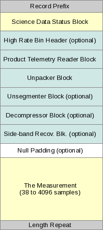
Figure 3.1: Science Data WGDS packets

All final science products delivered to the PDS are originally given to the Waves IOT as product telemetry files. These product telemetry files consist of pure Waves IDP packets without other padding or headers. By the time Waves data makes it through the Level 2 processing chain, packets have the layout defined in Figure 3.1. Though the Level 2 data packets contain many header blocks, most Level 3 products may be written using only the Science Data Status block. The Science data status block is key, as it identifies the receiver used to collect the measurement, the time of collection and the binary format of the samples in the data section.

3.1 Sample Vector Types (The PSID)

Waves generates only a limited number of different sample vectors. Each sample vector type has a unique Packet and Source ID (PSID). Many properties of the vector may be determined using the PSID and table 3.1 below. These include:

• the input sensor (electric, magnetic or spacecraft noise),
• the original sampling frequency,
• time domain to the frequency domain translations,
• amplitudes averaging in frequency space,
• the original data resolution (8-bit, 12-bit, 16-bit),
• mixing channel source (In-phase or Quadrature).

Properties that are not defined by the PSID are:

• sample vector start time,
• gain state of the pre-amp and receiver,
• mixer frequency,
• final data resolution.

3.2 Science Data Status Header Block

Program processing Level 2 data generate and update this header block. The Science Data Status Block defines the state of the data section and contains both permanent fields that are retained after all processing is complete and temporary fields required for intermediate processing states, only the permanent fields will be defined. This block has the lowest type ID so that it will always occur directly following the prefix.

This block acts an expanded version of the mini-packet header. Ideally the mini-packet header emitted by Waves would be reused for ground processing. The limitation in doing so is that the mini-packet headers transmitted from Waves are designed to be as small as possible and thus cannot describe unsegmented data. That being said, no information is lost, so the original telemetered mini-packet headers could be recreated via information encoded in the Science Data Status block, the Unsegmenter block and the High Rate Bin Header block, along with some knowledge of the instrument to C&DH communication protocol.

Science Data Status Block fields relevant to generating Level 3 data are described below:

Collect SCLK: The full 32-bit spacecraft SCLK at the time of the data collection, reconstructed using the IDP header SCLK and the individual mini-packet RTI fields. This is a 32-bit MSB first unsigned integer.

Collect RTI (Real Time Interrupt): The internal Waves scheduling clock runs at 40 Hz. Thus operations can be scheduled to occur at most 1/40th of a second. An RTI value of 0 represents a collection that began as the clock clicked to a new second, and a value of 39 is the last possible measurement start time in a second.

Avg: The number of original data captures averaged within the Waves instrument to arrive at this measurement. Warning: This value must be set in ground software and may be in error.

MPH0 through MPH7: An updated mini-packet header were all fields in the original mini-packet header that no longer accurate have been zero'ed out. In order to convert data samples to waveform or spectra measurements, software must at least read the ID, PATN, BGAIN, ATTN, SRC, BND and FMT bit fields. The bits are broken out as follows:

ID and SRC: The combination of these two fields identifies the hardware and software path within the Waves instrument from which the samples were collected. In C one can get the combined ID by:

PSID = (ID << 4) | SRC;

so the ID filed becomes the upper four bits and the SRC filed becomes the lower 4 bits. See Table 3.1 for an overview of most Waves science record types listed by PSID.

RTI: This is a combination of the 40Hz interrupt counter plus the SCLK as follows:

RTI field = (0x3FF & SCLK)*40 + rti

This field is used in conjunction with the IDP_SCLK to determine the Collect SCLK and Collect RTI pair, which are much more convenient to work with.

PATN: If 1 the pre-amplifier attenuator is on. The attenuation is 25dB for the Lo E and B LFR channels, and 20dB for LFR Hi E, HFR baseband and HFR down-mixed channels.

BATN: If 1 the back end LFR attenuator is on for the Hi and Lo E channels which adds 20dB of attenuation to the signal. This field should be ignored for HFR data.

SATN: The HFR-44 and HFR-45 receivers each contain a programmable attenuator. To determine the receiver attenuation present in the samples use the relation:

Rec. Attn = SATN * 2 dB.

This field should be ignored for LFR data.

BND: The HFR-44 and HFR-45 receivers use a local oscillator to down-mix E-field signals that vary too quickly to be directly sampled via the on-board A/D converters. This byte provides the setting for the local oscillator, when in use. This it it only meaningful for data derived from the HFR I& Q channels, which would be PSIDs 0x88, 0x89, 0x8C, 0x8D, 0xF1 and 0xF2. The values are:

• 0x00 - HFR receiver is in baseband, A/D converter runs at 7MHz

• 0x01 - HFR receiver is sweeping for log detection (Making HFR spectrum packets)

• 0x0C to 0xBF - Mixer setting in MHz.

Note that the mixer runs at four times the center frequency for HFR I/Q packets thus:

Center MHz = BND / 4.0

FMT: The measurement format, provides the binary format for the numeric samples in the data section of the packet. Note that the Waves central processor is a "little-endian" architecture, and all multi-byte measurements are stored with the least significant byte in the lowest address. Values for the FMT field found in process Waves science data packets are:

• 0x2 -- 32-bit LSB first IEEE floating point values

• 0x4 -- 8-bit unsigned integers

• 0xC -- 16-bit LSB first unsigned integers

• 0x1C -- 16-bit LSB first unsigned integers

3.3 Other Header Blocks

Parsing the fields defined in Section 2.2 above are sufficient to determine how to read most types of measurements. Further documentation on all the header fields may be found in the text document WAVESEDR/WAVESBLKS.TXT located in the DOCUMENT/WAVESEDR directory of the JNOWAV_0000 volume. In particular the High Rate Bin Header block is useful for gathering the Quality Factors generated by the Waves Instrument to signal to the spacecraft C&DH system which waveform captures should be telemetered to the ground.

3.4 Data Section

The data section of the WGDS packet mostly consists of pure samples strung end to end without padding. Some packets contain more than one kind of data product and must be handled as exceptions, see "Gotchas" below. To convert the samples to floating point numbers read the FMT field in the MPH 7 byte of the Science Data Status block in the WGDS header. Though it may appear otherwise, the Waves IOT did not intentionally bury the data format.

To convert these samples to physical units consult the calibration document WAVESCAL.HTM. In addition the labels for the individual calibration files in the JNOWAV_1000/CALIB directory contain quite a bit of descriptive text explaining exactly how each column and field is utilized.

Since all sample vectors that are transformed to frequency space are handled in the exact same way based on the PSID, frequency values are not included in the data section. Instead assign frequency bin values using one of the tables below.

This frequency down mapping is handled on-board and applies to packets with the PSID values 0x91, 0x92, 0xF0 and 0xF4. All these measurements were acquired using the low frequency channel low frequency receiver (LFR-Lo). The on-board processing is not actually an average but rather a sum. Thus before sending raw values for these packet to the calibration functions, divide the values by the number of bins indicated in Table 3.4 below.

This frequency down mapping is handled on-board and applies to packets with the PSID values 0x93 and 0xF5. All these measurements were acquired using the high frequency channel low frequency receiver (LFR-Hi). Like the LFR-Lo data, the on-board processing is not actually an average but rather a sum . Thus before sending raw values for these packet to the calibration functions, divide the values by the number of bins indicated in Table 3.5 below.

This frequency down mapping is handled on-board and applies to packets with the PSID values 0x5F, 0x5B, and 0xF5. All these measurements were acquired the baseband channel of one of the high frequency receivers ( HFR-45 Baseband, or HFR-46 Baseband). Again, like the LFR-Lo data, the on-board processing is not actually an average but rather a sum . Thus before sending raw values for these packet to the calibration functions, divide the values by the number of bins indicated in Table 3.6 below.

Packets with PSIDs 0xF0, 0xF4, and 0xF5 contain three different spectra. All data are stored as 32-bit IEEE floats in little endian byte order. Assuming the number of data samples is N (a number that is always divisible by 3), the data layout is as follows:

• Floats 0 to N/3: The Noise Mitigated Spectrum
• Floats N/3 to 2N/3: The Original Spectrum
• Floats 2N/3 to N: The Solar Panel Noise Spectrum

Packets with PSIDs 0xA0, 0xA4, and 0xA5 contain three different waveforms stacked end-to-end along with a set of coefficients from the Noise Mitigation algorithm. All data are stored as 32-bit IEEE floats in little endian byte order. Assuming the number of data samples is N (a number that is always divisible by 3), the data layout is as follows:

• Floats 0 to N/3: The Input Signal + Solar Panel Noise
• Floats N/3 to 2N/3: The Sampled Solar Panel Noise
• Floats 2N/3 to (N-32): The Noise Mitigated Waveform
• Floats N-32 to N: The noise reduction algorithm coefficients

3.5 Process for Converting from L2 to L3 data

Though it has already been described in VOLSIS.HTM Section 3.3.2, it is worth restating the Level 2 data to Level 3 processing procedure using terms defined in this document. An outline of the steps preformed in the conversion from Level 2 WGDS packets on the JNOWAV_0000 volume to Level 3 WAVES_SURVEY SPREADSHEET objects on the JNOWAV_1000 volume follows.

1. Spectra and attenuator calibration files are loaded from the JNOWAV_1000/CALIB directory.

2. All WGDS packets on the JNOWAV_0000 volume containing WAVES_SURVEY data for a single UTC day are loaded to memory.

3. All WGDS packets on the JNOWAV_0000 volume containing Housekeeping data for a single UTC day are parsed to find sub-second time adjustments.

4. All packet data is converted to 32-bit IEEE floats and calibrated to physical measurements. This includes basic calibration plus adjustments for attenuation.

5. Data collection SCLKs are pulled from the Science Data Status block of each WGDS packet. Housekeeping sub-second time adjustments are then added to these SCLK values, the resulting SCLK is sent to SPICE for conversion to SCETs.

6. All calibrated E-field packets are matched in SCET space in an attempt to define SPREADSHEET rows that contain complete sweeps from 50Hz to 41 MHz. Partial rows will be defined for packets that could not be aligned into a complete sweep.

7. Two primary WAVES_SURVEY products are written to the JNOWAV_1000 volume containing all primary measurements for a particular UTC day. One for E-field data and the other for B-field data.

8. If noise reduction diagnostic data were present, auxiliary product files are written to contain those data.

The equivalent processing for WAVES_BURST data follows.

1. 1.Waveform and attenuation calibration files are loaded from the JNOWAV_1000/CALIB directory.

2. All WGDS packets on the JNOWAV_0000 volume containing WAVES_BURST data for a single continuous high-rate recording session are loaded to memory.

3. All WGDS packets on the JNOWAV_0000 volume containing Housekeeping data for a single UTC day are parsed to find sub-second time adjustments.

4. All packet data is converted to 32-bit IEEE floats and calibrated to physical measurements. This includes basic calibration plus adjustments for attenuation.

5. Data collection SCLKs are pulled from the Science Data Status block of each WGDS packet. Housekeeping sub-second time adjustments are then added to these SCLK values, the resulting SCLK is sent to SPICE for conversion to SCETs.

6. All measurements for the continuous recording session are written to a single product file.

4. Housekeeping Packets

Figure 4.1: Waves Housekeeping WGDS Packets

Since housekeeping packets just happen to be fixed length, files containing housekeeping data may be defined via standard PDS labels. Thus, most of the information needed to view these records may be obtained by reading any one PDS label for a file with the name pattern WAV_YYYYDDD_HSK_VXX.DAT on the JNOWAV_0000 volume.

4.1 Sub-second Collect Time Adjustments

The Collect SCLK fields in the WGDS science data packets are not exactly the real spacecraft SCLK at the time of data collection. There is a sub-second offset from spacecraft seconds which changes very slowly compared to the data collection rate. To save space in the Science data stream this offset is not reported in the science IDP packets generated by Waves. Instead these offsets are emitted into the housekeeping stream. Thus, to determine data collections times to greater that 1 second accuracy, housekeeping data must be loaded. This field containing the offset is named SCLK_SUBSEC and is defined and described in all housekeeping product labels.

4.2 Micro-packets

The housekeeping packets contain both a fixed content 64-byte section, which is defined via standard PDS labels followed by a 64-byte variable content containing 4, 16-byte micro-packets. Micro-packets are touched on below, but to get the details on the the usefulness of each micro-packet type consult the University of Iowa document Juno/Waves Housekeeping Telemetry Formats Reference Manual, 98-90016 JPL/DRD SE-007-001A.

Each housekeeping packet ends with 4 micro packets. A micro-packet is 16 bytes long and has the following format.

The Type field identifies the content of bytes 4-15 in the micro-packet. The following types are defined.

• 0x11: C&DH hardware clock tracking statistics 1

• 0x12: C&DH hardware clock tracking statistics 2

• 0x14: C&DH hardware clock anomaly

• 0xA1: Waves FFT Engine Test Status

• 0xA2: Waves FFT Engine Error Status

• 0xA3: Waves FFT Engine watchdog status

• 0xB1: Last B-Field reported by FGM

• 0xC1: IEB trigger report

• 0xC2: IEB text label

• 0xD1: Waves Instrument power switch status

• 0xE1: Command Error Counter

• 0xF1: Waves reset status, and bus side select

• 0xF2: Waves ROM status

• 0xF3: Waves Hardware Versions, software kernel version

• 0xF4: Waves software kernel version time-stamp

• 0xF5: Clock Statistics

• 0xF7: Quick scan of 8-bit A/D converters

• 0xF8: Quick scan of 16-bit A/D converters

The sequence field increments for each micro packet added to the output buffer in the Waves kernel software. At the time a housekeeping packet is emitted, the last 4 micro-packets are dumped into the output stream. Since new micro-packets may not be present, the sequence field may be used to identify repeated micro-packets and ignore them.

The RTI field is produced in the same manner as the RTI field in Section 3.1, and records the time at which the micro-packet was added to the output buffer.