
Juno Mission -- Waves Investigation
Waves Standard Product
Data Record and Archive Volume
Software Interface Specification
98-60037
2nd Revision September 23rd, 2015
Prepared by
C. W. Piker
W. S. Kurth
chris-piker@uiowa.edu
william-kurth@uiowa.edu
Dept. of Physics & Astronomy
The University of Iowa
Iowa City, IA 52242

This document has been reviewed for export control and does
NOT contain technical information controlled under the International
Traffic in Arms Regulations (22 CFR 120-130).
 |
 |
Christopher W. Piker
Waves Archivist/Document Custodian |
William S. Kurth
Waves Lead Co-Investigator/Juno Archivist |
 |
 |
David Gell
JSOC Manager |
Raymond J. Walker
PDS/PPI Node Manager |
 |
 |
Reta Beebe
PDS/ATMOS Node Manager |
Michael New
PDS Program Scientist |
 |
 |
Bill Knopf
PDS Program Executive |
Tom Morgan
PDS Program Manager |
1 Introduction
This software interface specification (SIS) describes the format and
content of the Juno Waves Investigation (Waves) Planetary Data System (PDS)
data archive. It includes descriptions of the Standard Data Products and
associated meta data, and the volume archive format, content, and
generation pipeline.
1.1 Distribution list
Table 1.1: Distribution list
| Name | Organization | Email |
|---|
| Chris Piker | U. of Iowa | chris-piker@uiowa.edu |
| William Kurth | U. of Iowa | william-kurth@uiowa.edu |
| Steve Joy | UCLA/PDS/PPI | sjoy@igpp.ucla.edu |
| Joe Mafi | UCLA/PDS/PPI | jmafi@igpp.ucla.edu |
| Ray Walker | UCLA/PDS/PPI | rwalker@igpp.ucla.edu |
| David Gell | SwRI/JSOC | david.gell@swri.org |
Table 1.2: Document change log
| Change | Date | Affected portion |
|---|
| Initial template | 2010-01-15 | All |
| Waves IOT Draft | 2010-06-03 | All |
| Converted to 2 Volume Layout | 2011-07-15 |
Section 5 split to become 5 & 6 |
| Adjusted file names | 2011-12-01 |
File names for L3 volume updated |
| Adjustments after PDS 2nd review | 2012-06-04 | All |
| Adjustments after W. Kurth's review | 2012-06-18 |
All, except Appendices |
| Changed cal table name, new BURST products | 2012-06-25 |
Section 6.3, Section
6.5.2 |
| Added L2 product description | 2013-02-01 |
Appendix C |
| Final Edits for 1st Revision. | 2013-04-12 |
Sections 1 |
| Post-Review Lien Resolution Edits - 2nd Revision |
2015-09-23 | Sections 1, 2, 3, 4, 5, 6, 7, and C |
1.3 TBD items
Table 1.3 lists items that are not yet finalized.
Table 1.3: List of TBD items
| Item | Section(s) |
| Add instrument paper when it's available |
1.9 |
| Determine CATS like tool for tracking Juno Submissions and the
method by which JSOC will deliver data to PPI |
4.1 |
Table 1.4: Abbreviations and their meaning
| Abbreviation | Meaning |
| A/D |
Analog to Digital |
| ADC |
Analog to Digital Converter |
| ASCII |
American Standard Code for Information Interchange |
| ATLO | Assembly, Test and Launch Operations - Typically
refers to pre-launch ground testing. |
| CATS | Cassini Archive Tracking System |
| CCSDS | Consultative Committee for Space Data Systems |
| CD-ROM | Compact Disc -- Read-Only Memory |
| CDR | Calibrated Data Record |
| CFDP | CCSDS File Delivery Protocol |
| CODMAC | Committee on Data Management, Archiving, and Computing
|
| C&DH | Command and Data Handler -- Juno's central
electronic system |
| CRC | Cyclic Redundancy Check |
| DMAS | Data Management and Storage |
| EDR | Experiment Data Record |
| EFB | Earth Fly-By |
| FEI |
File Exchange Interface - a JPL provided software package |
| FFT | Fast Fourier Transform - An efficient digital algorithm
for calculating discrete Fourier transformations of a number series |
| GB | Gigabyte(s) |
| GSFC | Goddard Space Flight Center |
| HFR |
High Frequency Receiver - A section of the Waves main electronics |
| HK |
Housekeeping - instrument and spacecraft health and status
monitoring information |
| HRS | High Rate Science - Refers to science data collected at
higher rate than normal, antonym of LRS |
| HTML | Hypertext Markup Language |
| ICD | Interface Control Document |
| IOT | Instrument Operations Team |
| ISO | International Standards Organization |
| JADE | Jovian Auroral Plasma Distributions Experiment |
| JEDI | Jupiter Energetic Particle Detector Instrument |
| JIRAM | Jupiter InfraRed Auroral Mapper |
| JPL | Jet Propulsion Laboratory |
| JSOC | Juno Science Operations Center |
| LFR | Low Frequency Receiver - A section of the Waves main
electronics |
| LRS | Low Rate Science - Refers to science data collected at a
nominal rate, antonym of HRS |
| MAG | Magnetometer Instrument |
| MB | Megabyte(s) |
| MOS | Mission Operations System |
| MSB | Most Significant Byte First -- layout for multibyte
fields, colloquially called "big endian" |
| MWR | Microwave Radiometer Instrument |
| NAIF |
Navigation and Ancillary Information Facility (JPL) |
| NASA | National Aeronautics and Space Administration |
| NSSDC | National Space Science Data Center |
| ODL | Object Description Language |
| PDDU |
Power Distribution and Drive Unit - a Juno spacecraft component |
| PDS | Planetary Data System |
| PPI | Planetary Plasma Interactions Node (PDS) |
| SCET | Spacecraft Event Time |
| SCLK | Spacecraft Clock |
| SFTP | Secure File Transfer Protocol |
| SIS | Software Interface Specification |
| SOS | Science Operations System |
| SPDR |
Standard Product (Experiment and Pipeline) Data Record |
| SPICE |
Spacecraft, Planet, Instrument, C-matrix, and Events (NAIF data format)
|
| SPK | SPICE (ephemeris) Kernel (NAIF) |
| SwRI | Southwest Research Institute |
| TBC | To Be Confirmed |
| TBD | To Be Determined |
| UVS | Ultraviolet Spectrometer Instrument |
| ΔV-EGA | Earth Gravity Assist |
1.5 Glossary
Archive -- An archive consists of one or more data sets along with
all the documentation and ancillary information needed to understand and use
the data. An archive is a logical construct independent of the medium on which
it is stored.
Archive Volume -- A volume is a logical organization of directories
and files in which data products are stored. An archive volume is a volume
containing all or part of an archive; i.e. data products plus documentation
and ancillary files.
Archive Volume Set -- When an archive spans multiple volumes, they
are called an archive volume set. Usually the documentation and some ancillary
files are repeated on each volume of the set, so that a single volume can be
used alone.
Catalog Information -- High-level descriptive information about a
data set (e.g. mission description, spacecraft description, instrument
description), expressed in Object Description Language (ODL), which is
suitable for loading into a PDS catalog.
Data Product -- A labeled grouping of data resulting from a
scientific observation, usually stored in one file. A product label
identifies, describes, and defines the structure of the data. An example of a
data product is a planetary image, a spectral table, or a time series
table.
Data Set -- A data set is an accumulation of data products together
with supporting documentation and ancillary files.
Experiment Data Record -- An accumulation of raw output data from a
science instrument, in chronological order, with duplicate records removed,
together with supporting documentation and ancillary files.
Standard Data Product -- A data product generated in a predefined
way using well-understood procedures and processed in "pipeline" fashion. Data
products that are generated in a non-standard way are sometimes called special
data products.
1.6 Juno Mission Overview
Juno launched aboard an Atlas V rocket from Cape Canaveral Air Force
Station on August 5th 2011. The spacecraft uses a ΔV-EGA trajectory
consisting of a deep space maneuver on 12 September 2012 followed by an Earth
gravity assist on 9 October 2013 at an altitude of 500 km. Jupiter arrival is
on 5 July 2016 using a 107-day capture orbit prior to commencing operations
for a 1-(Earth) year long prime mission comprising 32 high inclination, high
eccentricity orbits of Jupiter. The orbit is polar (90° inclination) with
a periapsis altitude of 4500 km and a semi-major axis of 19.91 RJ
giving an orbital period of 10.9725 days.
During each orbit primary science data are acquired for approximately 12
hours centered on each periapsis. In addition fields and particles data are
acquired at low rates for the remaining apoapsis portion of each orbit.
Currently, 5 of the first 7 periapses are dedicated to microwave radiometry of
Jupiter's deep atmosphere with the remaining orbits dedicated to gravity
measurements to determine the structure of Jupiter's interior. All orbits will
include fields and particles measurements of the planet's auroral regions.
Data acquired during the periapsis passes are recorded and played back over
the subsequent apoapsis portion of the orbit.
Juno is spin stabilized with a rotation rate of 1 -- 5 revolutions per
minute (RPM). The planned spin rate varies during the mission: 1 RPM for
cruise, 2 RPM for science operations, and 5 RPM for main engine maneuvers. For
the radiometry orbits the spin axis is precisely perpendicular to the orbit
plane so that the radiometer fields of view pass through the nadir. For
gravity passes, the spin axis is aligned to the Earth direction, allowing for
Doppler measurements through the periapsis portion of the orbit. The orbit
plane is initially very close to perpendicular to the Sun-Jupiter line and
evolves over the 1-year mission.
Juno's instrument complement includes Gravity Science using the X and Ka
bands to determine the structure of Jupiter's interior; vector fluxgate
magnetometer (MAG) to study the magnetic dynamo and interior of Jupiter as
well as to explore the polar magnetosphere; and a microwave radiometer (MWR)
experiment covering 6 wavelengths between 1.3 and 50 cm to perform deep
atmospheric sounding and composition measurements. The instrument complement
also includes a suite of fields and particle instruments to study the polar
magnetosphere and Jupiter's aurora. This suite includes an energetic particle
detector (JEDI), a Jovian auroral (plasma) distributions experiment (JADE), a
radio and plasma wave instrument (Waves), an ultraviolet spectrometer (UVS),
and a Jupiter infrared auroral mapping instrument (JIRAM). The JunoCam is a
camera included for education and public outreach. While this is not a science
instrument, the Juno mission team plans to capture the data and archive them
in the PDS along with the other mission data.
1.7 SIS Content Overview
Section 2 describes the Waves instrument. Section 3 provides a data overview and defines the production methods
and schedule. Section 4 describes the data sets, data flow,
and validation. Section 5 describes the structure of the
archive volumes and contents of each file. Section 7
describes the file formats used in the archive volumes. Individuals
responsible for generating the archive volumes are listed in Appendix A. PDS-compliant label files for all Waves standard data
products are itemized and described in Appendix B, while
the operation of the HFR frequency down-mixers are described in Appendix
C.
1.8 Scope of this document
The specifications in this SIS apply to all archive volumes containing
Waves data products submitted for archive to the Planetary Data System (PDS),
for all phases of the Juno mission. Some sections of this document describe
parts of the Waves archive and archiving process that are managed by the PDS
archive team. These sections have been provided for completeness of
information and are not maintained by the Waves team.
1.9 Applicable Documents
- Planetary Data System Archive Preparation Guide, Version 1.1, JPL
D-31224, 08/29/2006.
- Planetary Data System Standards Reference, JPL D-7669, Part 2,
Version 3.8, 02/27/2009.
- Planetary Science Data Dictionary Document, Planetary Data System,
JPL D-7116, Version 1r65, 02/2007.
- Juno Mission Operations Concept Document, JPL D-35531, Version
Preliminary, 04/30/2007.
- Juno Science Data Management and Archive Plan, Version Final, JPL
D-34032, 08/26/2009.
- Juno Science Operations Center (JSOC), JSOC-IOT Interface Control
Document, Rev 3, 12029.02-JSOC_IOT_ICD-01
- Juno Mission SOC -- PDS Atmospheres Node/PPI Node Interface
Control Document, (In process - no JPL document number available at
this time)
- Juno Project -- Waves Investigation, Software Final Detailed
Design, 98-60013-Rev2, DRD No. SW-004 Item 002B
- Juno/Waves Housekeeping Telemetry Formats Reference Manual,
98-90016 DRD SE-007-001A
- Juno Waves Instrument Paper
Not complete, Reference will be provided when available, paper will
be provided on the volume if publisher allows inclusion.
1.10 Audience
This document is useful to those wishing to understand the format and
content of the Waves PDS data product archive collection. Typically, these
individuals would include scientists, data analysts, or software
engineers.
2 Waves Instrument Description
2.1 Science Objectives
One of the four overarching science objectives of the Juno mission is to
explore, for the first time, the three-dimensional structure of Jupiter's
polar magnetosphere and aurorae. The Waves investigation directly supports
this theme. The Wave science objectives supporting this overarching objective
are to (1) determine the nature of coupling between Jupiter's internal
magnetic field, the ionosphere, and the magnetosphere, (2) investigate and
characterize the three-dimensional structure of Jupiter's polar magnetosphere,
and (3) identify and characterize auroral processes at Jupiter. These main
objectives are further broken down into the following:
- Locate and determine the nature of the auroral acceleration region.
- Identify the major current systems coupling the magnetosphere to the
ionosphere.
- Determine the role wave-particle interactions play in the Jovian aurora.
- Measure radio and plasma wave phenomena (auroral hiss, electron and
ion phase space holes, auroral radio emissions, etc.) emission
characteristics (intensity, electric and magnetic fields) inside source
regions.
- Identify and characterize emission processes.
- Determine the fundamental differences between aurora associated with
- The breakdown of co-rotation in the middle magnetosphere
- The solar wind
- Io (or other Galilean satellite) flux tube
- Determine the beaming properties of Jovian radio emissions at high
latitudes.
- Determine the source locations for Jovian auroral radio emissions.
Additional issues to be addressed by the Waves investigation include (1)
the determination of dust flux in the region above the atmosphere and below
Jupiter's ring system at and near the Jovigraphic equator and (2) look for
lightning-generated whistlers.
The Waves instrument utilizes two sensors. For the detection of the
electric component of waves, an electric dipole antenna is used. The antenna
is mounted on the aft flight deck, centered under solar panel wing #1 which
has the Magnetometer boom at its end. Each element of the dipole is 2.8 m
long. The two elements are deployed shortly after launch in a plane that is
tilted aft of the aft flight deck by 45° and with a subtended angle
between the two elements of 120°. An electric preamp is housed at the
root of the two dipole elements. The symmetry axis of the dipole projected
into the aft flight deck plane is parallel to the Magnetometer solar panel.
The antenna pattern of the dipole for low frequencies is approximately a
dipole with maximum sensitivity to electric fields parallel to the Y-axis of
the spacecraft, i.e. perpendicular to both the MAG boom axis and the spin
axis.
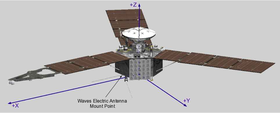
Figure 2.1: Spacecraft Coordinate System
(Origin of
the spacecraft frame is centered on the bottom at the launch vehicle
separation plane)
For the detection of the magnetic component of waves, a magnetic search
coil (MSC) is used. The search coil consists of a rod of mu-metal (permalloy)
material 15 cm long with 10,000 turns of copper wire on a bobbin surrounding
the rod. The coil is attached to the aft flight deck with its preamplifier
mounted close by. The long axis of the MSC is parallel to the spacecraft Z
axis (along the high gain antenna axis), hence, the antenna pattern is
approximately that of a dipole with maximum sensitivity parallel to the spin
axis of the spacecraft. This configuration minimizes the variation of signal
at the spin frequency.
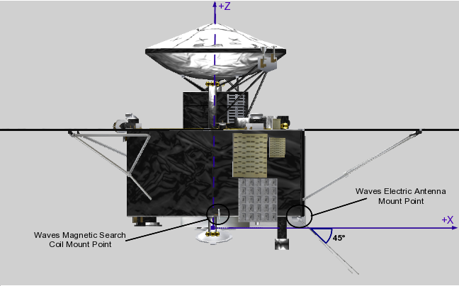
Figure 2.2: Waves Sensor Mounting Points
(Spacecraft +Y axis is into the page)
The Waves electronics (other than the preamplifiers mentioned above) reside
in the main electronics box in the Juno radiation vault. A simple block
diagram of the instrument is provided in Figure 2.2.
There are three receivers.
The Low Frequency Receiver (LFR) comprises two identical low-frequency
channels (LFR-Lo) covering the range from 50 Hz to 20 kHz and allows
measurements of both the electric and magnetic component of waves (utilizing
both sensors). A third channel in the LFR (LFR-Hi) analyzes signals only from
the electric dipole and covers the frequency range of 10 to 150 kHz. The
outputs from the two LFR-Lo channels are digitized waveforms consisting of 50
ksps at 16 bit resolution. The waveforms are sent to the Digital Signal
Processor (DSP) for spectrum analysis. The output from the LFR-Hi channel is
digitized at a rate of 375 ksps with 16 bit accuracy. This waveform is also
analyzed by the DSP.
Utilizing signals from the electric dipole, the High Frequency Receivers
(HFR) are capable of covering the range from 100 kHz to 45.25 MHz, though
typical science data cover the range from 137 kHz to 41 MHz. The baseband
channel of each HFR (100 kHz -- 3 MHz) is a broadband channel that is sampled
at a rate of 7 Msps with 12 bit resolution. To cover the frequency range
above 3 MHz, a synthesized frequency is mixed with the incoming signals and
the resulting combined signal is filtered to remove components above 500 kHz.
This down-mixes high frequency information that was within 1 MHz of the
synthesized frequency into the 0 to 0.5 MHz range. The mixed signal may be
measured via two different analog signal pathways depending on the desired
resolution of the data products. Each receiver may be used to generate low
resolution survey data products or higher resolution burst products. The
HFR-44 receiver is tuned to step it's internal frequency synthesizer slightly
faster than the other HFR and is typically used to produce survey products,
though either receiver may be commanded to produce either product type.
Survey HFR data records are produced in the 100 kHz to 3 MHz
range by sending the output of the baseband channel (7 Msps at 12-bit
resolution) to the Waves DPU for spectrum analysis. The resulting data
products covering the range of 137 kH to 2.98 MHz in 27 logarithmically spaced
frequency bins. To produce survey data records above 3 MHz, the power in each
1 MHz band is recorded via a log amplifier whose output is sampled with 8 bit
resolution. Power levels are collected sequentially as in a swept frequency
receiver. Though the instrument may be commanded to set the center
frequency of these 1 MHz bands as high as 44.75 MHz, standard HFR science
operations are conducted with a top mixer frequency of 40.5 MHz and thus a
41 MHz top edge for the detection range.
Burst HFR data records are gathered when Juno passes near or
through the source regions of Jovian radio emissions. Since these data
have a much higher frequency and time resolution not all bands are collected
on a regular cadence. Instead only the band which overlaps the electron
cyclotron frequency. Band selection is driven by magnetic field values
received from the Magnetometer once per 2 seconds. Using
fce = 28*|B| where fce is the electron cyclotron frequency in Hz and |B| is
the magnitude of the magnetic field in nT, a 1-MHz band including fce is
selected for waveform measurements. This is because the Jovian auroral radio
emissions are generally believed to be generated via the cyclotron maser
instability very close to fce.
Unlike the Survey HFR value, all burst HFR products are waveforms. The
baseband waveforms samples (7 Msps) are stored as is, without reduction in
the DPU. High-frequency (above 3 MHz) science products are not derived from
log amplifier measurements. Instead two internally synthesized signals are
mixed with the incoming signal from the electric preamp. Both synthesized
signals are at the same frequency but second signal is phase shifted by 90
degrees relative to the first. As in the survey measurement case, the
resulting combined signals are filtered below 500 kHz but instead of
measuring the the power of the entire band, both are sampled at 1.3125 Msps
with 12-bit resolution for storage and transmission. This sampling rate is
more than twice the Nyquist frequency of the down-mixed signal. Further
processing of the two simultaneous waveforms is preformed on the ground to
separate the upper and lower sidebands and produce a high resolution 1 MHz
spectrogram centered on the mixer frequency. The specific processing
algorithm required to separate frequency components is provided in
Appendix C.
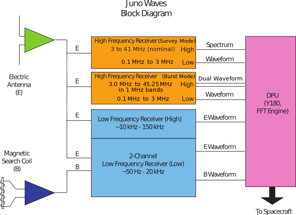
Figure 2.3: Waves Block Diagram
The Digital Signal Processor serves both as a spectrum analyzer for the
waveforms from the various receivers as well as the data processing unit for
the Waves instrument, receiving and acting on commands from the spacecraft as
well as building and transmitting data packets to the spacecraft. The DPU
consists of a Y180 processor core and various utility functions implemented in
a field-programmable gate array (FPGA) and a fast Fourier transform (FFT)
engine implemented in a second FPGA. The FFT engine can be considered as a
floating point arithmetic unit under control of the Y180 processor. The
signal processing tasks of the DPU include controlling the A/D converters in
the various receivers, collecting waveforms, running lossless Rice compression
on waveforms (in the case of burst waveform data which is to be sent to the
ground without spectrum analysis), Fourier transforming the waveforms, binning
and averaging the resulting Fourier components, and optionally performing
noise cancellation of the LFR-Lo and LFR-Hi signals.
Juno Waves returns two types of data products. The instrument produces a
magnetic spectrum from 50 Hz to 20 kHz and an electric spectrum from 50 Hz to
41 MHz at a regular cadence, depending on where it is in orbit about Jupiter.
During perijove passes, nominally the 12 hours centered on Jupiter closest
approach, the cadence is a full magnetic and electric spectrum every second.
For most of the remainder of the orbit, the cadence is a spectrum every 30
seconds. An intermediate rate mode has been defined for specific intervals,
such as just outside perijove and for plasma sheet crossings near apojove,
which has a cadence of one spectrum per 10 seconds.
The second type of data product consists of waveforms from the various
receivers. The waveform products are obtained by compressing the waveforms
from one or more of the Wave analysis bands in the LFR and possibly one from
an HFR during commanded burst modes (see below for a description of the
burst modes).
All digital LFR survey measurements as well as the HFR Baseband survey
measurements begin as waveform samples within the receivers. LFR data are
collected via 16-bit ADCs and HFR baseband measurements are made using 12-bit
Analog to Digital conversion. In each case 6144 samples are collected at the
sample rate given in Table 6.8. These are then
transformed via a hardware FFT algorithm as 6 individual 1024 point time series
with no overlap and then autocorrelated. The lower half of the 6 spectra
autocorrelations are averaged resulting in a single 512 point spectra. The
spectra values are binned in frequency into logarithmically spaced set. Each
receiver band uses a different frequency bin table. The binning tables are
defined in the "Juno Project -- Waves Investigation, Software Final
Detailed Design" document referenced in section 1.9.
Finally, to preserve telemetry bandwidth while maintaining a large dynamic
range, the value of each bin is converted to a 9-bit floating point number
before transmission to the Juno spacecraft C&DH system. Details of the
9-bit float format can also be found in the previous reference.
The upper bands of the HFR (3 to 41 MHz) are sampled much like a traditional
sweep frequency receiver. The power in a 1 MHz band is recorded via an 8-bit
ADC and saved as a single byte value. No further manipulations are preformed
on these measurements in-flight.
Compared to Survey data, Burst mode values undergo relatively few
manipulations within the instrument. LFR burst measurements as well as HFR
baseband burst measurements are typically collected as 6144 point time series.
The LFR waveforms are sampled with 16-bit resolution while the HFR baseband
is sampled with 12-bit resolution. After collection, the time series are
compressed using the lossless Rice compression algorithm and transmitted to
the C&DH.
HFR burst measurements above 3 MHz are pairs of 1024 point time series
collected simultaneously at 12-bit resolution from the output of the in-phase
and quadrature mixers. These pairs are also passed through a lossless Rice
compression algorithm and transmitted to the C&DH. Further processing
is required to unambiguously assign amplitude values to frequencies. These
details are provided in Appendix C of this document.
It is the intention of the Waves Instrument Operations Team (IOT) to
conduct science activities using the following instrument modes.
2.5.1 Survey Modes
Waves has three survey (or low-rate) modes.
2.5.1.1 Perijove mode
During perijove passes, nominally the 12 hours centered on Jupiter closest
approach, the cadence is a full magnetic and electric spectrum every second.
2.5.1.2 Apojove mode
For most of non-perijove portion of the orbit, the cadence is a spectrum
every 30 seconds.
2.5.1.3 Intermediate mode
An intermediate rate mode has been defined for specific intervals, such as
just outside perijove and for plasma sheet crossings near apojove, which has a
cadence of one spectrum per 10 seconds.
Waves has two types of burst modes.
2.5.2.1 Binning mode
In this mode, when enabled, Waves looks for intense, broadband signatures
of crossings of auroral field lines carrying a host of intense wave modes. It
continuously sends burst mode data, usually from LFR-Lo (E and B), LFR-Hi, and
the tuned HFR band including fce to the Command and Data Handling (C&DH)
system which stores them in two or more buffers sized to hold approximately a
minute's worth of waveform data (although this length and the number of
buffers is selectable). Waves also characterizes such broadband bursts with a
quality factor (defined below), which the C&DH uses to determine whether
to keep or over-write a buffer. At the end of the binning session, the
buffers with the highest quality factor (QFactor) will be formatted by the
C&DH for transmission to the ground. JADE will normally participate in
Binning mode burst periods in conjunction with Waves. The two instruments
will have the same number of buffers defined for a binning session with
lengths that are designed to record similar (time) durations of high rate
data. The Waves quality factors will be used to identify which of the JADE
buffers are kept, as well, so that both instruments have high rate burst data
for approximately the same intervals.
Binning mode QFactors are calculated using survey data. While this may
seem counter intuitive for a waveform product it is a straight forward
operation for the onboard software. As explained in Section
2.4.1 above, all LFR survey products, as well as all HFR baseband survey
products, are generated via an on-board FFT of time series waveforms along
with some binning of the resulting spectral value autocorrelations. To
calculate the QFactor for a set of waveform measurements, a program in the DPU
adds the exponents of a programmed set of LFR and/or HFR baseband bins
together. The sum of the exponents is then scaled by a constant to put the
resulting value into the range of 1 to 128. For a single binning session all
QFactors are derived from the same set of frequency bins. However the
selection of frequency bins used to calculate the qfactor may change from one
binning session to another. Thus QFactors are useful as a relative measure of
spectral power within a single binning session but comparison of QFactors
across binning sessions requires careful consultation of the instrument
command logs to insure that no changes to the QFactor frequency set have been
introduced.
2.5.2.2 Record mode
In this mode, a single buffer is defined and waveform data from one or more
of the Waves receivers are recorded for a commanded interval of time. This
mode was designed with crossings of the Jovian equator near perijove in mind.
Typically data from just the LFR-Lo (E) channel will be recorded to be used to
identify micron-sized dust particle impacts with the spacecraft as Juno
crosses the ring plane.
While both burst modes were designed with specific Jovian observations in
mind, either can be used at any time and for any purpose, including distant
plasma sheet crossings or simply for instrument checkout.
Waves is part of the Juno auroral suite of instruments and is scheduled to
be on basically for the entire prime mission, both the Gravity and MWR orbits.
Waves' power requirements vary with data production and the data volume
afforded Waves is limited, hence, it is not possible for Waves to be in
perijove mode for large portions of the orbit and burst modes are even more
restricted. Since in burst mode Waves can generate data at about 1 Mbps, and
a nominal data volume allocation for Waves is limited to about 2 Gigabit per
orbit, burst mode usage is limited to only a few minutes of each orbit. These
are typically divided among the northern and southern auroral crossings and an
equator crossing. The event quality determination algorithm is parametrized
and it is anticipated that a fair amount of experimentation with these
parameters in the early orbits will be required to tune them for optimum
use.
The bulk of the Waves calibrations are carried out on the ground prior to
integration on the spacecraft with spot checks of these carried out during
ATLO. The calibrations involve precisely measuring the gains of the
preamps and gain amplifiers (and attenuators) in the receivers, the filter
responses of each of the receivers, the transfer function of the search coil,
and the base capacitance of the electric preamp. The ultimate goal of the
calibrations is to be able to accurately relate the telemetered values to
physical field strengths and spectral densities.
Waves carries no in-flight calibration signal, hence, the possibilities for
in-flight calibration are limited. For past wave instruments, in-flight
calibrations have been attempted using radio signals (such as solar type III
radio bursts) simultaneously observed by another space borne receiver, although
such a calibration is fraught with uncertainties and will likely only serve to
confirm that the instrument calibration has not drifted significantly.
Another calibration possibility is using the galactic background as a
calibration source. This was performed on the Cassini RPWS data with good
success. However, with the short Juno antennas and the likelihood of
significant spacecraft EMI, it is unlikely that Waves will be able to detect
the galactic background.
One significant calibration is planned for flight. This has to do with
using Waves data to perform limited direction-finding measurements on Jovian
radio signals. Since the Waves electric antenna rotates with the spacecraft,
a null will be seen in the electric field signal when the dipole axis
(spacecraft Y axis) is most closely pointed toward the source. Said another
way, Waves will be able to determine the plane containing the source and the
spacecraft spin (Z) axis. This could be quite useful near Jupiter over the
poles when the distance to sources are small and the motion of the spacecraft
provides a range of perspectives to a given source, even though it does not
replicate the 2-dimensional direction-finding capability of multi-antenna
instruments such as that on Cassini. In order to carry out the so-called
'rotating dipole' direction-finding technique, it is necessary to accurately
determine the beaming pattern of the antenna. This is done while on approach
to Jupiter when Jupiter is far enough from Juno such that the location of the
radio sources with respect to the direction of Jupiter can be assumed to be a
small angle, yet close enough that the Jovian radio emissions are reliably
detectable. The useful distance range for this calibration is thought to be
between about 400 and 100 Jovian radii (RJ), subject to the
in flight noise levels including spacecraft electromagnetic interference.
The standard product types generated by the Waves IOT as well as which
volumes contain those types are listed in Tables 3.1 and
3.2. See section 6.3.2 of the Planetary Data System
Standards Reference for definition of the data processing levels. This
document will only use the CODMAC processing level designation.
Together the HK, LRS, and HRS data sets include all Waves science and
housekeeping data. These products consist of raw instrument data packets that
have been minimally and reversibly transformed along with the instrument
housekeeping data. These data are included for completeness and as a way to
re-generate higher level products if necessary. They are not intended for
general use. The SURVEY, and BURST products provide the same data coverage at
the same resolution in a much more usable form. Only minimal PDS labels will
be accompany these products, though complete documentation will be provided in
the volume's DOCUMENT directory.
The data set ID for these raw products is:
JNO-E/J/SS-WAV-2-EDR-V1.0.
Table 3.1: Volume JNOWAV_0000 Data Products
| Standard Data Product ID |
Content |
NASA Level |
CODMAC |
Processing Inputs |
Product Format |
Filename Token |
| HK |
Housekeeping Data Records |
0 |
2 |
Housekeeping data from the DMAS |
Binary TABLEs |
_HSK_ |
| LRS |
Decompressed, Unsegmented EDRs |
0 |
2 |
Level 2 low rate science data from the DMAS |
Binary FILEs |
_LRS_ |
| HRS |
Decompressed, Unsegmented EDRs |
0 |
2 |
Level 2 high rate science data from the DMAS |
Binary FILEs |
_HRS_BIN_
_HRS_REC_ |
Level 3 products consist of two product sets, SURVEY and
BURST. The SURVEY products consist of calibrated electric
and magnetic spectral density measurements collected via the LFR and HFR
receivers at the sampling rates given in Table 6.8.
This is a full resolution data set that will include all spectra received
from Waves, from launch to end of mission.
The data set ID for SURVEY products is:
JNO-E/J/SS-WAV-3-CDR-SRVFULL-V2.0.
BURST products consist of electric and magnetic waveforms primary
collected via the LFR and HFR receivers during auroral and equatorial
crossings. These waveforms are filtered and sampled at a variety of
frequencies as listed in Table 6.9. All waveforms from
launch to end-of-mission are to be included in the BURST data set.
The data set ID for BURST products is:
JNO-E/J/SS-WAV-3-CDR-BSTFULL-V2.0.
Table 3.2: Volume JNOWAV_1000 Data Products
| Standard Data Product ID |
Content |
NASA Level |
CODMAC |
Processing Inputs |
Product Format |
Primary Filename Tokens |
| SURVEY |
Wave amplitudes vs.
frequency and time |
1B |
3 |
HK and LRS data products
Spice Spacecraft Clock kernel
Calibration Tables
Mission Phase and Orbit boundaries
|
ASCII SPREAD-SHEETs |
_E_
_B_ |
| BURST |
Time-ordered waveforms,
Wave amplitudes vs.
frequency and time |
1B |
3 |
HK and HRS data products
Spice Spacecraft Clock kernel
Calibration Tables
Mission Phase and Orbit boundaries
|
Binary TABLEs |
_E_BIN_
_E_REC_
_B_BIN_
_B_REC_
_NBS_BIN_
_NBS_REC_ |
The Juno Data Management and Storage (DMAS) system will receive packets and
CCSDS File Delivery Protocol (CFDP) products from the Deep Space Network (DSN)
and place these on the Project data repository system. The DMAS will provide
the initial processing of the raw telemetry data bringing it to Committee on
Data Management and Archive (CODMAC) Level 2 science data, comprising bested
and de-overlapped data. At this point compressed data are not decompressed.
The Waves Instrument Operations Team (IOT) will retrieve the CODMAC Level 2
data from the DMAS using FEI services and ancillary data from the JPL Mission
Support Area (MSA) via Juno Science Operations Center (JSOC). The Waves IOT
will decompress the Level 2 data, where necessary, and deliver them to the
JSOC. The JSOC will also receive and organize higher level data products
developed by the Science Investigation Teams associated with each instrument.
JSOC development and operations will be carried out at SwRI, in coordination
with the MOS at JPL.
Once science Experiment Data Records, or EDRs (CODMAC Level 2 data), have
been produced by the JPL MOS they will be transferred to the Instrument
Operation Team. Decompression of compressed data and any necessary
restructuring of the data will be carried out by the Waves IOT. The Waves
Science Investigation Team will verify the content and the format will be
validated. The resulting decompressed, restructured Level 2 data will
constitute the lowest level of data to be archived with the PDS. While not the
most useful data for the community, these uncalibrated data comprise a data
set of last resort, should later, irreversible processing errors be discovered
at some later date. JSOC will coordinate the validation of the edited (CODMAC
Level 2) data archive products created by the Waves IOT. The Science
Investigation Team will develop higher level data products based on the Level
2 data and ancillary data and return these to the JSOC. JSOC will support
archiving the Level 2 data by building archive volumes and verifying the
format of the volumes and included data and metadata. Higher level data set
archives will be coordinated through the JSOC. The Science Investigation Team
will be responsible for ensuring that the metadata and documentation included
with these data sets are complete and accurate. This means that both JSOC and
the Science Investigation Team will need to work closely with the PDS. This
coordination will be fostered via the Data Archive Working Group.
A comprehensive description of the Juno Mission System is provided in the
Juno Mission Operations Concept. A data flow diagram for the downlink process
is shown in Figure 3.1. In the figure, White boxes are
processes and solid arrows indicate data flow.
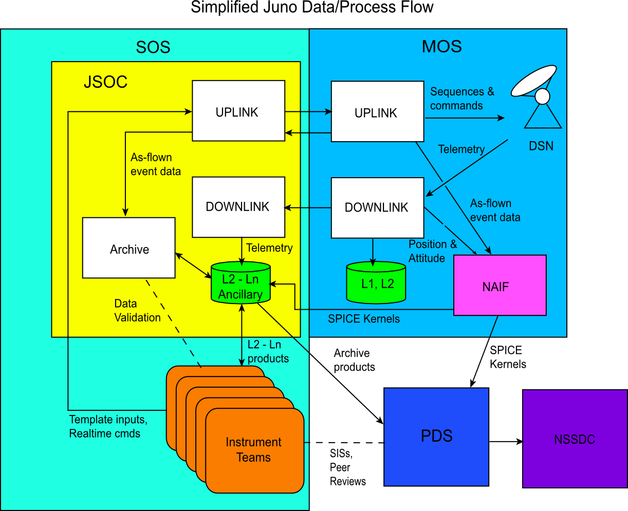
Figure 3.1: Juno science data flow diagram
Raw science and housekeeping data files are automatically transferred to
the Waves IOT via an FEI subscription registered with the DMAS. From these
inputs, and local calibration data, PDS products are produced automatically
for inclusion in the JNOWAV_0000 and JNOWAV_1000 archive volumes.
The basic unit of output for the Waves instrument is a packet. Each
product file transferred to the Waves IOT from the DMAS is simply a set of
instrument packets concatenated end-to-end without meta-data. Since packets
do not have a one-to-one correspondence with EDRs, the purpose of the Level 2
data production pipeline is to reversibly recover individual measurements from
instrument generated packets.
For each science and housekeeping file set the following operations are
preformed:
- CRC Validation -- For each instrument packet, ground calculated CRCs are
compared against instrument generated CRCs. Packets which do not pass CRC
validation are skipped.
- Sorting -- Packets from all file sources for a specified time frame are
sorted by SCET into a single list using the SCLK - SCET correlation is
provided by project supplied SPICE kernels.
- Unpacking -- To save telemetry bandwidth, Waves drops redundant
measurement headers. This processing step copies headers as appropriate.
- Unsegmentation -- Measurements that are too long to fit within length
constraints of the Juno flight data system are segmented into multiple output
packets by Waves. In this processing step these segmented measurement are
reassembled.
- Decompression -- Waves has the capability to compress data prior to
output. In this step measurements are decompressed as necessary.
- CRC Regeneration -- A new CRC is generated for each EDR using the same
algorithm as the Waves instrument.
- Label Generation -- PDS labels are generated for each output file. Each
label includes the MD5 hash of the associated data file.
- The local JNOWAV_0000 volume index is updated. Label file MD5 hashes
are stored in the index file.
- EDR Transmission -- The unsegmented, decompressed reformatted experiment
data records (EDR) and Housekeeping data are delivered to the JSOC via SFTP.
Both SURVEY and BURST products are produced as follows:
Extraction -- Level 2 science EDRs are scanned for instrument generated survey
mode spectra, and burst mode waveforms. During extraction, CRCs are
recalculated for each EDR and compared to the encoded value. If the
calculated value is not the same as the encoded value processing is halted and
operator intervention is required as this may indicate an error in the Level 2
data product or the Level 2 data processing pipeline.
Fine time offsets are located in the Level 2 housekeeping records.
Calibration -- The best known calibration is applied to each point in
the spectra and waveform data.
SCET application -- The most up to date Spice Spacecraft Clock kernel
is used to convert the SCLK with the fine time offset to spacecraft event
time.
Output -- PDS data files are generated containing the calibrated data.
In the case of survey mode data, PDS SPREADSHEET objects are generated. For
burst mode waveforms, PDS SERIES objects are generated.
Label Generation -- PDS labels are generated for each output file.
Each label includes the MD5 hash of the associated data file.
The local JNOWAV_1000 volume index is updated. Label file MD5
hashes are stored in the index file.
CDR Transmission -- The Calibrated Data Record (CDR) files are
delivered to the JSOC via SFTP.
Products submitted to the JSOC and to PDS will be validated via
automatic software checks and routine use.
Waves generates and transmits a Cyclic Redundancy Check (CRC) field with
each packet. Though CRCs can not absolutely guarantee that data were not
altered in transmission, they require relatively little processing time and do
provide reasonable assurance of data integrity. The Level 2 data processing
pipeline validates each packet's CRC, logging and dropping any packets which
fail. In addition each EDR output by this pipeline carries a newly generated
CRC. The Level 3 pipeline halts on CRC failure, forcing operator intervention
and correction. Finally each PDS product label carries an MD5 checksum for
the associated product data file.
In addition to these transmission integrity checks, basic data sanity
checks are to be built into the production pipelines. The following
conditions will automatically alert the Waves IOT.
1.Raw data contains zeros not indicated in the transmission log file.
2.Data is at the noise floor and gain control is not at maximum.
3.Data is clipped.
No doubt others will be added as the mission evolves. At a minimum these
checks will affect the data quality index, in extrema cases, individual EDRs
and CDRs may be excluded from higher level data sets.
Finally alarms in instrument housekeeping records may indicate invalid
blocks of science data records. These will be considered on a case-by-case
basis.
Waves investigators will use the same files for their science analyses as
are archived with the PDS. Further, other Juno scientists will access and use
these same files from JSOC prior to archiving for their analyses. The Waves
investigators have found repeatedly that the best way to validate science data
is to use the data for science analyses. In accordance with the principle of
"use what you archive":
Level 3 products shall be generated from archived Level 2 products.
Browse images shall be generated from archived Level 3 products.
All display and analysis software created or modified for Waves
investigators shall use level 3 PDS products.
We believe this plan will result in the best validation of the products
before they are archived.
In the event that a data file or range of data files are determined to be
in error, one of two courses of action are possible. If the error is
discovered prior to releasing the data to PDS, new files containing the
revised data will be submitted to the JSOC and the old file will be removed.
If an error is discovered in data released to the PDS, new files are submitted
to the JSOC, then JSOC will then re-summit the new files to PDS for
validation.
In either case, all replacement science data files shall increment the
version number in the file name, and in the PRODUCT_VERSION_ID element of
the associated PDS label.
The processing pipelines are 'cron' jobs that will execute once every hour
to check for and process new data received via FEI subscriptions from the
DMAS. Pipeline generated errors will be handled on a daily basis or ASAP by
the Waves archivist. The Waves Science Team will review data products on a
daily basis.
The Waves Standard Data Record archive collection is produced by the Waves
IOT in cooperation with the JSOC, and with the support of the PDS Planetary
Plasma Interactions (PPI) Node at the University of California, Los Angeles
(UCLA). The archive volume creation process described in this section sets out
the roles and responsibilities of both these groups. The assignment of tasks
has been agreed by both parties, and codified herein. Archived data received
by the PPI Node from the Waves IOT will be made electronically available to
PDS users as soon as practicable but no later than as laid out in
Table 4.1.
Data products delivered to PDS will accrue on one of two volumes. Raw data
products will be added to volume JNOWAV_0000, while the much more useful
full-resolution, calibrated science products become part of the JNOWAV_1000
volume.
The Waves IOT will deliver data to the JSOC. JSOC will transfer the data
to the PPI Node in standard product packages containing three months of data,
also adhering to the schedule set out in Table 4.1. Each
package will comprise both data and ancillary data files organized into
directory structures consistent with the volume design described in
Section 5, and combined into a deliverable file(s) using
file archive and compression software. When these files are unpacked at the
PPI Node in the appropriate location, the constituent files will be organized
into the archive volume structure.
Table 4.1: Archive Schedule and Responsibilities
| Data Product (CODMAC) |
Volume |
Provider |
Earth Flyby |
Other Cruise |
Orbital Phase |
| HK, LRS, HRS (level 2) |
JNOWAV_0000 |
Waves, C.W. Piker |
EFB + 18 months |
Jupiter + 4 months |
EDA + 3 to 6 months |
| BURST, SURVEY (level 3) |
JNOWAV_1000 |
Waves, C.W. Piker |
EFB + 18 months |
Jupiter + 4 months |
EDA + 3 to 6 months |
EFB -- Earth Flyby, EDA -- End of data acquisition
The archive products will be sent electronically from the Waves IOT to the
JSOC using the SFTP protocol. JSOC, acting as an agent of the Waves
Investigating Team, will transfer the data to the PPI node. The IOT operator
will copy volume files (see Table 4.3) to an appropriate
location within the JSOC file system. Only those files that have changed since
the last delivery will be included. The JSOC operator or software will run
basic validation checks as defined in the JSOC-IOT Interface Control
Document, 12029.02-JSOC_IOT_ICD-01. JSOC will transfer the contents of
the data delivery to the PPI node using the process defined in the "Juno
Mission SOC -- PDS Atmospheres Node/PPI Node Interface Control Document". Each
step of data submission process will be due to be tracked in a TBD version of
CATS (Cassini Archive Tracking System) which has been adapted for use by
Juno.
Following receipt of a data delivery, PPI will organize the data into PDS
archive volume structure within its online data system. PPI will generate all
of the required files associated with a PDS archive volume (index file,
read-me files, etc.) as part of its routine processing of incoming Waves data.
Newly delivered data will be made available publicly through the PPI online
system once accompanying labels and other documentation have been validated.
It is anticipated that this validation process will require at least fourteen
working days from receipt of the data by PPI. The first two data deliveries
are expected to require somewhat more time for the PPI Node to process before
making the data publicly available.
All PDS data are subject to Peer Review under the auspices of the PDS. Data
acquired during the Earth flyby was the pathfinder data set for PDS archiving.
Early cruise data, including Earth flyby, were the first to undergo peer
review Processing this initial data-set has taken likely longer than the
pipeline flow expected during the prime mission at Jupiter. The peer review
has validated the data processing pipelines, the SIS, and all data formats and
meta-data. It is anticipated that subsequent archive deliveries will be
subjected to content and format validation by both the science team and the
PDS, but that a formal peer review panel will not be required.
The archiving schedule is defined in Table 4.1 and
is designed to be consistent with the archiving schedule in the Juno Science
Data Management and Archive Plan.
The Waves standard data archive volume set will include all data acquired
during the Juno mission. The archive validation procedure described in this
section applies to volumes generated during both the cruise and prime phases
of the mission.
PPI node staff will convene a peer review panel consisting of PDS personnel
and likely data users outside the Juno Mission. The panel will review the
first versions of the archive volumes containing data from the Earth Flyby to
determine whether the archive is appropriate to meet the stated science
objectives of the instrument. The peer panel will also review the archive
product generation process for robustness and ability to detect discrepancies
in the end products; documentation will be reviewed for quality and
completeness.
Additionally, the Waves team may generate and archive special data products
that cover specific observations or data-taking activities. This document does
not specify how, when, or under what schedule, any such special archive
products are generated. It is assumed this SIS would be revised to include
such additional data sets and/or products.
Waves standard data products are organized into files that span one Earth
solar day or less, breaking at 0h UTC. Files vary in size depending on the
telemetry rate and allocation. Table 4.2 summarizes the
expected sizes of the Waves standard products. Burst data will be packaged in
files individually covering the three (typically) burst mode collections per
orbit (North auroral crossing binned data, Equator crossing recorded data, and
South auroral crossing binned data). In addition to one-day files, it is
anticipated that tools will be provided on the Level 3 volume (JNOWAV_1000)
in the EXTRAS directory to display and output periapsis survey data
covering the ~12-hours of periapsis data collection.
All Waves standard data are organized by the PDS team onto two archive
volumes. The products on the L2 raw data volume are to be organized in to one
sub-directory per 100 Earth solar days and then into one sub-directory per
Earth solar day. The data on the L3 calibrated science data
volume are to be organized into sub-directories by mission phase and after
Jupiter capture, by orbit number, and then into one sub-directory per Earth
solar day. Following receipt of Waves data by the PPI Node it is expected
that fourteen working days will be required before the data are made available
on PPI web pages.
The PPI Node keeps three copies of each archive volume. The primary copy is
the version maintained online at UCLA, and distributed through the PPI
webpages. A second copy is stored locally on an offline disk. The third copy
is on an off-site mirror maintained at the University of Iowa. Once the
archive pipeline has been fully validated, copies of the data products will be
periodically transmitted by PPI to the National Space Science Data Center
(NSSDC) for long-term archive in a NASA-approved deep-storage facility. The
PPI Node may maintain additional copies of the archive volumes, either on or
off-site as deemed necessary. The process for the dissemination, and
preservation Waves archive volumes is illustrated in Figure
4.1.

Figure 4.1: Duplication and dissemination of Waves
standard archive volumes.
Each Waves data volume bears a unique volume ID using the last two
components of the volume set ID (PDS Standards Reference, section 19.1). The
volume IDs are USA_NASA_PDS_JNOWAV_nnnn, where JNOWAV is the VOLUME_SET_ID
defined by the PDS and nnnn is either 0000, for the raw data volume, or 1000
for the calibrated science data volume. This is summarized in
Table 4.3.
Table 4.3: PDS Data Set Name
Assignments
| CODMAC |
DATA_SET_ID |
VOLUME_ID |
| Level 2 |
JNO-E/J/SS-WAV-2-EDR-V1.0 |
USA_NASA_PDS_JNOWAV_0000 |
| Level 3 |
JNO-E/J/SS-WAV-3-CDR-SRVFULL-V2.0 |
USA_NASA_PDS_JNOWAV_1000 |
| Level 3 |
JNO-E/J/SS-WAV-3-CDR-BSTFULL-V2.0 |
USA_NASA_PDS_JNOWAV_1000 |
The JNOWAV_0000 volume contains the safed Experiment Data Records (EDRs)
from the Juno Waves instrument starting from launch though the end of mission.
Though an organized raw data collection is prudent, this volume is not
intended for use by the wider public and is thus minimally described. All
files defined in this section, except those specifically noted, are to be
provided by the Waves IOT. The complete directory structure is shown in Figure 5.1
.
Figure 5.1: Archive volume directories
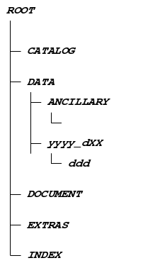
The files listed below are contained in the (top-level) root directory, and
are produced by the Waves team in consultation with the PPI node of the PDS.
With the exception of the hypertext file and its label, all of these files are
required by the PDS volume organization standards.
Table 5.1: ROOT directory contents
| File Name |
File Description |
| AAREADME.HTM |
This file completely describes the volume organization and contents.
|
| AAREADME.LBL |
A PDS detached label that describes AAREADME.HTM |
| AAREADME.TXT |
This file completely describes the volume organization and contents (PDS
label attached) |
| ERRATA.TXT |
A text file containing a cumulative listing of comments and updates
concerning all Waves EDR products on all JNOWAV_0000 volume versions published
to date. |
| VOLDESC.CAT |
A description of the contents of this volume in a PDS format readable by
both humans and computers |
The files in the CATALOG directory provide a top-level understanding of the
Juno mission, spacecraft, instruments, and data sets in the form of completed
PDS templates. The information necessary to create the files is provided by
the Waves team and formatted into standard template formats by the PPI Node.
The files in this directory are coordinated with PDS data engineers at both
the PPI Node and the PDS Engineering Node.
Table 5.2: CATALOG directory contents
| File Name |
File Description |
| CATINFO.TXT |
A description of the contents of this directory |
| DATASET.CAT |
PDS data set catalog description of the HK, LRS and HRS EDRs
(PPI Node shares responsibility for this file) |
| INSTHOST.CAT |
A description of the Juno Spacecraft
(Supplied by Juno Project)
|
| MISSION.CAT |
PDS mission catalog description of the Juno mission
(Supplied by
Juno Project) |
| PERSON.CAT |
PDS personnel catalog description of Waves team members and other persons
involved with generation of Waves standard data products |
| PROJREF.CAT |
References mentioned in INSTHOST.CAT and MISSION.CAT
(Supplied by
Juno Project) |
| WAVESINST.CAT |
PDS instrument catalog description of the Waves instrument |
| WAVESREF.CAT |
Waves related references mentioned in other CATALOG files |
The DATA directory contains the data files produced by the Waves IOT for
the standard product types; HK, LRS and HRS. Together these data set consists
of raw binary instrument reformatted experiment data records (EDRs) and
housekeeping data, organized into correct time sequence, time tagged, and
edited to remove obviously bad data. All data files are of the highest
quality possible. Any residual issues are documented in AAREADME.TXT and
ERRATA.TXT. Users are referred to these files for a detailed description of
any outstanding matters associated with the archived data. Additional files
relevant to the data files are located in the EXTRAS/SEQUENCE sub-directory
(see Section 6.7).
Table 5.3: DATA directory contents
| Item Name |
Item Description |
| DATAINFO.TXT |
A file describing the of the contents of this directory. |
| YYYY_DXX |
Sub-directories containing raw instrument Experiment Data Records (EDRs)
and housekeeping data. Each sub-directory all EDRs for SCET year "yyyy" and
hundred day, day-of-year block beginning with digit "d". For example,
2011_2XX includes the range 2011-200T00:00:00.000 (Midnight, July 19) up to,
but not including, 2011-300T00:00:00.000 (Midnight, October 27). |
This directory tree contains the standard products, HK - Housekeeping, LRS
- Low Rate Science, and HRS - High Rate Science telemetry packets. Though this
data set is not intended for general use, steps have been taken to place the
science data in a more usable form. Since much of the Waves data is
compressed within the instrument, this data set includes uncompressed data so
that a user would not have to determine how to correctly decompress the
different types of data using different compression schemes. Also, since the
Waves telemetry packets include a secondary level of organization referred to
as minipackets (a Waves minipacket includes telemetry from a single receiver
for a given interval of time, usually a measurement cycle), and since a single
measurement cycle can be segmented - split across minipackets, we have
unsegmented these and made sure that all data for a given measurement cycle
are one cohesive structure. Because of these simplifications, the reformatted
telemetry packets are not fixed length and their individual fields can not be
described by current PDS labels. Also, since all of these data are archived
as calibrated records with standard PDS labeling elsewhere, we have included
only minimal PDS labels for the science data files. The WAVESEDR.HTM
document within the DOCUMENT directory provides information on how to extract
and use data from this data set, should that extraordinary circumstance arise.
Unlike its science counterpart, waves housekeeping telemetry is inherently
fixed length, though it has its own complications. The first half of each
housekeeping record contains a fixed structure. The second half includes
optional information whose field definitions can change from record to record.
Thus we have labeled housekeeping data sufficiently to allow the fixed
portion to be read automatically by PDS software tools such as NASAView, and
tbtool. The optional fields are described in the University of Iowa document,
98-90016: Juno/Waves Housekeeping Telemetry Formats Reference Manual.
In order to manage files in an archive volume more efficiently, and assist
users who are manually locating products, the DATA directory is divided into
sub-directories as listed in Figure 5.1. A simple
"1 directory equals 1 SCET day" scheme is employed.
A PDS label describes each file in the DATA path of an archive volume. Text
documentation files have attached (internal) PDS labels and data files have
detached labels. Detached PDS label files have the same root name as the file
they describe but have the extension LBL.
Products in this directory make up the JNO-E/J/SS-WAV-2-EDR-V1.0 data set,
which includes both science and housekeeping telemetry. As shown in
Table 5.4, data in the housekeeping and survey mode files
span an interval of one day, the particular day is indicated in the file name.
The file name also includes a file version number. These are included for
tracking reissued data, should the need arise. As required, each file is
accompanied by a PDS label (LBL) describing its contents. In the file name
patterns below yyyy is the year, ddd is the day of year, hh is the hour of the
day, mm is the minute of the hour, and ss is the second of the minute, and nn
is the product version number, starting at 01.
Table 5.4: DATA/yyyy_dXX/ddd
subdirectory contents
| File Name Pattern |
Standard Product ID |
File Description |
| WAV_yyyyddd_HSK_Vnn.DAT |
HK |
This pattern is used for daily
housekeeping data files. All housekeeping packets whose report time is
within the day are included within the file. |
| WAV_yyyyddd_HSK_Vnn.LBL |
HK |
Labels for files with the pattern Tyyyyddd_HSK_Vnn.DAT.
Housekeeping packets start with an fixed format 64 bytes portion followed by
a variable content 64 byte portion. Since PDS labels do not have the required
flexibility to describe the variable content portion, these labels only
provide sufficient information to extract fields from the initial 64 bytes of
each housekeeping packet. |
| WAV_yyyyddd_LRS_Vnn.PKT |
LRS |
This is a daily level 2 Low Rate Science file. All low rate raw science
EDRs, regardless of the instrument mode, whose measurement start times are
within the day are included in the file. |
| WAV_yyyyddd_LRS_Vnn.LBL |
LRS |
Rudimentary PDS labels for WAV_yyyyddd_LRS_Vnn.PKT files. Due
to the inability of PDS labels to describe variable length structures these
labels merely define a file object and point to the appropriate documentation.
|
| WAV_yyyydddThhmmss_HRS_BIN_Vnn.PKT |
HRS |
Files with this pattern contain waveforms selected on-board via a
desirability algorithm. Here yyyy is the year, ddd is the
day of year (1st day has the value 1), hh is the hour of day,
mm is the minute of the hour, ss is the second of the
minute, and nn is the version number. The coverage period of these
files varies based on the size of the burst mode bin specified in the
controlling activity sequence. |
| WAV_yyyydddThhmmss_HRS_BIN_Vnn.LBL |
HRS |
Rudimentary PDS labels for WAV_yyyydddThhmmss_HRS_BIN_Vnn.PKT
files. Due to the inability of PDS labels to describe variable length
structures these labels merely define a file object and point to the
appropriate documentation.
|
| WAV_yyyydddThhmmss_HRS_REC_Vnn.PKT |
HRS |
Files with this pattern contain waveforms recorded over a pre-selected
time period without regard for the data content. The coverage period of these
files varies based on the length of the sequenced record mode session. |
| WAV_yyyydddThhmmss_HRS_REC_Vnn.LBL |
HRS |
Rudimentary PDS labels for WAV_yyyydddThhmmss_HRS_REC_Vnn.PKT
files. Due to the inability of PDS labels to describe variable length
structures these labels merely define a file object and point to the
appropriate documentation.
|
The DOCUMENT directory contains a range of documentation considered either
necessary or useful for users to understand the archive data set. Documents
may be provided in ASCII, HTML, or PDF format, though PDS standards require
that any documentation needed for use of the data be available as plain text.
HTML is acceptable as a plain text. The following files are contained in the
DOCUMENT directory, grouped into the sub-directories shown.
Table 5.5: DOCUMENT directory contents
| File Name |
Description |
| DOCINFO.TXT |
A description of the contents of this directory tree |
| VOLSIS/VOLSIS*.PNG |
Graphics files used by VOLSIS.HTM |
| VOLSIS/VOLSIS.LBL |
A detached label for the HTML and PDF versions of this document |
| VOLSIS/VOLSIS.PDF |
This document in PDF |
| VOLSIS/VOLSIS.HTM |
This document as HTML text with minimal markup. |
| WAVESINST/WAVESINST.LBL |
A detached label for the PDF and HTML versions of the instrument document
|
| WAVESINST/WAVESINST.HTM |
A description of the Waves instrument in HTML text with minimal markup
|
| WAVESINST/WAVESINST.PDF |
A description of the Waves instrument in PDF |
| WAVESINST/IMAGE*.PNG |
Graphics files used by WAVESINST.HTM |
| WAVESEDR/WAVESEDR.LBL |
A detached label for the raw packet document. |
| WAVESEDR/WAVESEDR.HTM |
Raw Waves packet documentation as HTML text with minimal markup |
The EXTRAS directory is reserved for items that, while deemed useful
enough to include on the volume, are outside the scope of PDS archive
requirements. One item of note is a collection of the commands send to
the Waves instrument. These are stored in the EXTRAS/SEQUENCE directory.
These files are a bit cryptic and no attempt has been made to define nor
explain their contents. Other content may be added to EXTRAS over the course
of the mission. Consult the EXTRINFO.TXT file on each version of
the JNOWAV_0000 volume for more information on any items contained within
this directory.
The INDEX.TAB file contains a listing of all data products on the archive
volume. The index (INDEX.TAB) and index information (INDXINFO.TXT) files are
required by the PDS volume standards. The format of these ASCII files is
described in Section 7.2.6. An online and
web-accessible index file will be available at the PPI Node while data volumes
are being produced. As the Waves IOT plans to release updates to single
comprehensive volumes, there is no need for a CUMINDX.TAB file within the
INDEX directory.
Table 5.6: INDEX directory contents
| File |
Description |
| INDXINFO.TXT |
A description of the contents of this directory |
| INDEX.LBL |
A PDS detached label that describes INDEX.TAB |
| INDEX.TAB |
A table listing all Waves data products on this volume |
This section describes the contents of the Waves standard product
archive collection volume, JNOWAV_1000, including the file names, file
contents, and file types. All files, except those specifically noted, are to
be provided by the Waves IOT. The major directory structure is shown in
Figure 6.1. The top-level sub-directories of
BROWSE, DATA/WAVES_SURVEY, DATA/WAVES_BURST in the
figure below begin with a date. These dates denote the beginning of the
associated mission phase or Jupiter orbit. Since it is desirable to break up
this level of the archive by mission phase (during cruise) and then by orbit
(during the prime mission), date prefixes were added so that these items
appear in time order in most file browsers.
All ancillary files described herein appear on each volume revision. Because
Waves data releases are handled by releasing entire revised volumes, not by
providing companion volumes containing only new data, each release must
constitute a complete set of information.
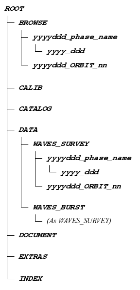
Figure 6.1: Archive volume directories
The files listed below are contained in the (top-level) root directory, and
are produced by the Waves team in consultation with the PPI node of the PDS.
With the exception of the hypertext file and its label, all of these files are
required by the PDS volume organization standards.
Table 6.1: ROOT directory contents
| File Name |
File Description |
| AAREADME.HTM |
This file completely describes the volume organization and contents, it
also contains links to the volume's graphical data browser. |
| AAREADME.LBL |
A PDS detached label that describes AAREADME.HTM |
| AAREADME.TXT |
This file completely describes the volume organization and contents (PDS
label attached) |
| ERRATA.TXT |
A text file containing a cumulative listing of comments and updates
concerning all Waves standard products on all Waves volumes in the volume set
published to date |
| VOLDESC.CAT |
A description of the contents of this volume in a PDS format readable by
both humans and computers |
The BROWSE directory contains frequency-time spectrogram images in Portable
Network Graphics (PNG) generated from the SURVEY and BURST data products.
Though each image is generated from full resolution data, the rendering
process often involves combining multiple measurements into a single pixel.
Thus browse images typically contain less information in the time domain for
SURVEY data and less information in the frequency domain for BURST data than
the input data products. Multiple data points are reduced by simple averaging
when necessary.
Browse data have been divided into cruise and orbit categories so that the
subdirectory layouts may be tailored to each situation. Layout and coverage
periods are detailed in subsequent sections.
Table 6.2: BROWSE directory contents
| Item Name |
Item Description |
| BROWINFO.TXT |
A file describing the of the contents of this directory |
| yyyyddd_ORBIT_xx |
Sub-directory for browse images for data collected during a single
Jupiter orbit. This storage scheme is used after Jupiter orbit insertion.
|
| yyyyddd_phase_name |
Sub-directory for browse images for data collected during a single mission
phase. Sub-directories further divided plots by Earth solar day. This
storage scheme is used to store cruise data, including Earth flyby plots.
|
This directory contains all browse plots generated from data collected
during a single Jupiter orbit. For the file name patterns in
Table 6.3, yyyy, ddd, hh,
mm, and ss denote the year, day of year, hour of day,
minute of hour and second of minute of the starting coverage period of the
data products used to generate the plot. Thus data may not start an the time
point given in the file name. Plot file versions are indicated by
nn and match the highest version number of the input data
products. For the periapsis survey plots, xx is the number of
the orbit containing the periapsis pass.
Table 6.3: BROWSE/WAVES_SURVEY/YYYYDDD_ORBIT_xx
directory contents
| Source Product Type |
File Name Pattern |
File Description |
| SURVEY |
WAV_yyyydddThhmmss_SRV_Vnn.PNG
WAV_yyyydddThhmmss_SRV_Vnn.LBL |
Survey mode magnetic field spectrogram from 50 Hz to 20 kHz and electric
field spectrograms from 50 Hz to 41 MHz spanning a single Earth solar day
|
| SURVEY |
WAV_PERI_xx_SRV_Vnn.PNG
WAV_PERI_xx_SRV_Vnn.LBL |
Survey mode magnetic field spectrogram from 50 Hz to 20 kHz and electric
field spectrograms from 50 Hz to 41 MHz spanning roughly 12 hours, centered on
periapsis |
| BURST |
WAV_yyyydddThhmmss_BST_150K_Vnn.PNG
WAV_yyyydddThhmmss_BST_150K_Vnn.LBL |
High frequency resolution electric field spectrograms spanning
50 Hz to 150 kHz and a magnetic field spectrogram from 50 Hz to 20 kHz,
of up to 20 minute duration |
| BURST |
WAV_yyyydddThhmmss_BST_45M_Vnn.PNG
WAV_yyyydddThhmmss_BST_45M_Vnn.PNG |
High frequency resolution, electric field spectrograms spanning the range
of 135 Hz up to 45.25 MHz, of up to 20 minute duration
|
In each orbit directory are spectrograms generated from SURVEY
products. There is one survey spectrogram per Earth solar day, or partial
Earth solar day per orbit. In addition, an extra survey image is included
which "zooms in" to the periapsis pass. Periapsis images cover roughly a
12 hour period centered on Jupiter closest approach.
Each orbit sub-directory also contains frequency-time spectrograms
generated from the BURST products. Compared to survey mode browse
data, each spectrogram image depicts a much shorter time span at higher
frequency and time resolutions. Since these data are typically acquired for
brief intervals with long time intervals in between, there will be one file
for each acquisition interval, unless another acquisition interval follows
within 20 minutes, in which case the time range of the burst spectrograms may
extend up to 20 minutes in duration. Typically the time component of the
browse plot file names matches the time component of the input product file.
In cases where more than one product file contribute data to the browse plot
the time of the first file is used.
Cruise browse images are stored in directories such as these. The contents
of this directory tree are very similar to the YYYYDDD_ORBIT_xx directories
above with the exception that only a single day's images with be contained
within a single directory instead of a multi-day orbital period. For the
top level cruise directories, YYYYDDD is the day on which the mission phase
starts, and yyyy_ddd is a sub-directory named for a single day within the
phase. In this way directories naturally sort in time order. Though the
directory dates align with mission phases, daily subdirectories only exist
during periods when Waves is operating. There are large blocks of time
when Waves was shutoff during cruise.
Each daily subdirectory contains only a single SURVEY plot but
there are as many BURST plots as needed to present all the burst mode
sessions that were initiated on the associated UTC day. The coverage period
for each survey file is a single solar day beginning at 0h UTC. Coverage
periods for the burst plots are the same as described in
Section 6.2.1 above. Unlike orbit directories, burst
data collection periods may extend across directory boundaries during cruise.
In these instances BURST plots are placed in the daily directories
corresponding to the beginning of their associated data product's
coverage period, and thus the first plotted information may actually
correspond to a UTC day different from that denoted on the filename.
Table 6.4: BROWSE/YYYYDDD_phase_name/yyyy_ddd
directory contents
| Source Product Type |
File Name Pattern |
File Description |
| SURVEY |
WAV_yyyydddThhmmss_SRV_Vnn.PNG
WAV_yyyydddThhmmss_SRV_Vnn.LBL |
Survey mode magnetic field spectrogram from 50 Hz to 20 kHz and electric
field spectrograms from 50 Hz to 41 MHz, spanning a single Earth solar day
|
| BURST |
WAV_yyyydddThhmmss_BST_150K_Vnn.PNG
WAV_yyyydddThhmmss_BST_150K_Vnn.LBL |
High frequency resolution electric field spectrograms spanning
50 Hz to 150 kHz and a magnetic field spectrogram from 50 Hz to 20 kHz,
of up to 20 minute duration |
| BURST |
WAV_yyyydddThhmmss_BST_45M_Vnn.PNG
WAV_yyyydddThhmmss_BST_45M_Vnn.PNG |
High frequency resolution, electric field spectrograms within the
range of 135 Hz up to 45.25 MHz, of up to 20 minute duration
|
The CALIB directory contains the ancillary data used to calibrate the Waves
instrument. These tables are used with the HK, LRS, and
HRS CODMAC level 2 products from the JNOWAV_0000 volume to
produce the level 3 data sets on this volume. Though they are not expected to
change often, all of the calibration table files below carry a version number,
indicated as nn, starting with 01. The contents of this directory are
described in the following table.
Table 6.5: CALIB directory contents
| File Name Pattern |
File Description |
| CALINFO.TXT
|
A description of the contents of this directory |
WAV_CAL_ATTN_Vnn.CSV
WAV_CAL_ATTN_Vnn.LBL
|
Defines the attenuation values corresponding to a given state of the
Electric Preamp and the Receivers. Preamp and receiver states change from
packet to packet, but the relationship between a given state and it's
signal attenuation is fixed. |
WAV_CAL_BST_DIRECT_AMP_Vnn.CSV
WAV_CAL_BST_DIRECT_AMP_Vnn.LBL
|
The calibration table used to produce the directly sampled BURST mode
electric and magnetic field amplitude products volume. Waveforms sampled at
50kHz, 375kHz, and 7 MHz are calibrated at a mid-band frequency using
coefficients from these files. |
WAV_CAL_BST_NBS_AMP_Vnn.CSV
WAV_CAL_BST_NBS_AMP_Vnn.LBL
|
The mid-band amplitude calibration coefficients for BURST mode 1MHz wide
spectra products produced from down-mixed electric waveform samples. |
WAV_CAL_BST_NBS_FREQ_Vnn.CSV
WAV_CAL_BST_NBS_FREQ_Vnn.LBL
|
Frequency response adjustments to the amplitude calibrations for BURST
mode 1MHz wide spectra products produced from down-mixed electric waveform
samples. Normalizations included in these files have not been applied
to the data but the table has been included for completeness in the case that
it may be useful. |
WAV_CAL_SRV_HFR_HI_44_Vnn.CSV
WAV_CAL_SRV_HFR_HI_44_Vnn.LBL
|
A look-up table providing the conversion for instrument values to
physical units for measurements collected via the electric antenna, filtered
through one of the HFR upper bands, down mixed via a local oscillator,
integrated over a set time period, and sampled once per channel. |
WAV_CAL_SRV_HFR_HI_45_Vnn.CSV
WAV_CAL_SRV_HFR_HI_45_Vnn.LBL
|
A look-up table providing the conversion for instrument values to
physical units for measurements collected via the electric antenna, filtered
through one of the HFR upper bands, down mixed via a local oscillator,
integrated over a set time period, and sampled once per channel. |
WAV_CAL_SRV_HFR_LO_44_Vnn.CSV
WAV_CAL_SRV_HFR_LO_44_Vnn.LBL
|
A look-up table providing the conversion from instrument values to
physical units for measurements collected via the electric antenna, filtered
through the HFR base band, sampled at 7 MHz and then digitally converted to
spectra. |
WAV_CAL_SRV_HFR_LO_45_Vnn.CSV
WAV_CAL_SRV_HFR_LO_45_Vnn.LBL
|
A look-up table providing the conversion from instrument values to
physical units for measurements collected via the electric antenna, filtered
through the HFR base band, sampled at 7 MHz and then digitally converted to
spectra. |
WAV_CAL_SRV_LFR_HI_E_Vnn.CSV
WAV_CAL_SRV_LFR_HI_E_Vnn.LBL
|
A look-up table providing the conversion from instrument values to
physical units for measurements collected via the electric antenna, filtered
through the LFR high band, sampled at 375 kHz and then digitally converted to
spectra. |
WAV_CAL_SRV_LFR_HI_N_Vnn.CSV
WAV_CAL_SRV_LFR_HI_N_Vnn.LBL
|
A look-up table providing the conversion from instrument values to
physical units for measurements collected via the spacecraft power supply
noise input, filtered through the LFR high band, sampled at 375 kHz and then
digitally converted to spectra. |
WAV_CAL_SRV_LFR_LO_B_Vnn.CSV
WAV_CAL_SRV_LFR_LO_B_Vnn.LBL
|
A look-up table providing the conversion from instrument values to
physical units for measurements collected via the magnetic search coil,
filtered through the LFR low band, sampled at 50 kHz and then digitally
converted to spectra. |
WAV_CAL_SRV_LFR_LO_E_Vnn.CSV
WAV_CAL_SRV_LFR_LO_E_Vnn.LBL
|
A look-up table providing the conversion from instrument values to
physical units for measurements collected via the electric antenna, filtered
through the LFR low band, sampled at 50 kHz and then digitally converted to
spectra. |
WAV_CAL_SRV_LFR_LO_N_Vnn.CSV
WAV_CAL_SRV_LFR_LO_N_Vnn.LBL
|
A look-up table providing the conversion from instrument values to
physical units for measurements collected via the spacecraft power supply
noise input, filtered through the LFR low band, sampled at 50 kHz and then
digitally converted to spectra. |
WAV_CAL_SRV_HFR_HI_PROP_Vnn.CSV
WAV_CAL_SRV_HFR_HI_PROP_Vnn.LBL
|
Provides the center frequencies and noise bandwidths for the upper bands
of the high frequency receivers. |
WAV_CAL_SRV_HFR_LO_PROP_Vnn.CSV
WAV_CAL_SRV_HFR_LO_PROP_Vnn.LBL
|
Provides the center frequencies and noise bandwidths for the digital
spectra channels from the baseband frequency path within the HFR receivers.
|
WAV_CAL_SRV_LFR_HI_PROP_Vnn.CSV
WAV_CAL_SRV_LFR_HI_PROP_Vnn.LBL
|
Provides the center frequencies and noise bandwidths for the digital
spectra channels from the high frequency path within the LFR receiver. |
WAV_CAL_SRV_LFR_LO_PROP_Vnn.CSV
WAV_CAL_SRV_LFR_LO_PROP_Vnn.LBL
|
Provides the center frequencies and noise bandwidths for the digital
spectra channels from the low frequency path within the LFR receiver. |
The files in the CATALOG directory provide a top-level understanding of the
Juno mission, spacecraft, instruments, and data sets in the form of completed
PDS templates. The information necessary to create the files is provided by
the Waves team and formatted into standard template formats by the PPI Node.
The files in this directory are coordinated with PDS data engineers at both
the PPI Node and the PDS Engineering Node.
Table 6.6: CATALOG directory contents
| File Name |
File Description |
| BURST_DS.CAT |
PDS data set catalog description of the WAVES_BURST products
(PPI Node shares responsibility for this file) |
| CATINFO.TXT |
A description of the contents of this directory |
| INSTHOST.CAT |
A description of the Juno Spacecraft
(Supplied by Juno Project)
|
| MISSION.CAT |
PDS mission catalog description of the Juno mission
(Supplied by
Juno Project) |
| PERSON.CAT |
PDS personnel catalog description of Waves team members and other persons
involved with generation of Waves standard data products |
| PROJREF.CAT | References mentioned in INSTHOST.CAT and
MISSION.CAT
(Supplied by Juno Project) |
| SURVEY_DS.CAT |
PDS data set catalog description of the WAVES_SURVEY products
(PPI
Node shares responsibility for this file) |
| WAVESINST.CAT |
PDS instrument catalog description of the Waves instrument |
| WAVESREF.CAT |
Waves related references mentioned in other CATALOG files |
The DATA directory contains the data files produced by the Waves IOT for
the standard product types; SURVEY and BURST. The SURVEY data set consists of
ASCII comma-separated-values files that result from passing the corresponding
HK and LRS product files through the CDR data processing pipeline (see
Section 3.3.2). The BURST data set consists of binary
data files that are also generated from the CDR pipeline but where HK and HRS
products are the inputs. All data files are of the highest quality possible.
Any residual issues are documented in ERRATA.TXT and the CONFIDENCE_NOTE
section in the BURST_DS.CAT and SURVEY_DS.CAT catalog files. Users are
referred to these files for a detailed description of any outstanding matters
associated with the archived data.
Table 6.7: DATA directory contents
| Item Name |
Item Description |
| DATAINFO.TXT |
A file describing the of the contents of this directory. |
| WAVES_SURVEY |
Sub-directory for standard resolution electric and magnetic field spectra
making up the standard SURVEY data products. |
| WAVES_BURST |
Sub-directory containing electric and magnetic field waveforms making up
the standard BURST data products. |
The Waves Level 3 archive contains both SURVEY and BURST standard products.
SURVEY mode products contain spectra at a lower frequency resolution than
those provided by ground processing of BURST products. Due to telemetry
bandwidth limitations BURST products are only available for selected time
periods, while SURVEY products are generated whenever the Waves instrument is
operating.
For SURVEY products the LFR and HFR receivers are run a regular cadence
that usually allows a single row of an E field spectra data file to contain a
complete set of measurements, running from 50 Hz to 41 MHz. Magnetic field
spectra data files contain a complete set of measurements running from 50 Hz
to 20 kHz. The SURVEY products intended for the archive user are those with
"_E_" and "_B_" as part of the file name. Though other files are present and
these bear explanation.
In an attempt to remove interference from the spacecraft power system the
Waves instrument can be commanded into a noise mitigation mode. When noise
mitigation is enabled the LFR samples signals from the spacecraft Power
Distribution and Drive Unit (PDDU) as well as each sensor. Using both the
signal from the sensor as well as the signal from the PDDU a noise-mitigated
spectrum is calculated. Nominally only the noise-mitigated spectrum or the
unaltered spectrum is transmitted to the ground, though Waves can be commanded
to down-link all three spectra (original sensor signal, noise signal, noise
canceled signal). In this case three files will be present for each sensor
for each day as given in Table 6.8.
Table 6.8 summarizes the types of SURVEY products.
Note the difference between the highest frequency electric field survey data
and the rest. Unlike the lower frequency bands, the high frequency survey
mode data are generated in steps. The A/D converters within the instrument
are not capable of running at the rates needed to directly sample waveforms
above 3 MHz. To measure electric waves at higher frequencies the input signal
is down mixed with a signal generated within the HFR receiver. The amplitude
level of the resulting mixed signal is recorded via a simple log-amplifier,
not an A/D converter. The mixer frequency is adjusted 38 times during a single
sweep of the HFR to produce the upper frequency survey mode data.
Table 6.8: SURVEY Standard Product Summary
| File Mnemonic |
Standard Product ID |
Contents & Sensor |
Input Filters |
Sampling Rates |
Onboard FFT |
_E_
(primary file) |
SURVEY |
Noise-mitigated electric field spectra if available, if
noise-mitigation is not enabled then this file contains uncorrected electric
field spectra. |
50Hz-20kHz |
50kHz |
Yes |
| 10kHz-150kHz |
375kHz |
| 100kHz-3MHz |
7MHz |
| Stepped from 3MHz to 41MHz. |
N/A |
No |
_EUNC_
(secondary file) |
SURVEY |
Serves as a storage location for uncorrected spectra when
noise-mitigated spectra are using up the 'E' file slot. |
50Hz-20kHz |
50kHz |
Yes |
| 10kHz-150kHz |
375kHz |
_EINT_
(secondary file) |
SURVEY |
PDDU Interference spectra, when available. |
50Hz-20kHz |
50kHz |
Yes |
| 10kHz-150kHz |
375kHz |
_B_
(primary file) |
SURVEY |
Noise-mitigated magnetic filed spectra if available, if noise-mitigation
is not enabled then this file contains uncorrected magnetic field spectra.
|
50Hz-20kHz |
50kHz |
Yes |
_BUNC_
(secondary file) |
SURVEY |
Serves as a storage location for uncorrected spectra when noise-mitigated
spectra are using up the 'B' file slot. |
50Hz-20kHz |
50kHz |
Yes |
_BINT_
(secondary file) |
SURVEY |
PDDU Interference spectra, when available. |
50Hz-20kHz |
50kHz |
Yes |
Table 6.9 summarizes the various types of BURST
products. Except for the "_NBS_" products, these contain waveforms
generated via the various Waves A/D converters. These data have not been
transformed to frequency space on-board, nor have the component amplitudes
been combined into spectral bands. The narrow band spectra files, denoted
by the file mnemonic "_NBS_", are a bit different. These are generated by
combining each set of in-phase and quadrature waveforms on the ground
via the algorithm given in Appendix C. The resulting
spectra are centered at the mixing frequency and cover a 1.3125 MHz range, of
which only 1 MHz is within the pass band. The outer edges of the spectra are
outside the range of analog filters within the receiver. Note that "_NBS_"
data are only provided as spectra, the source waveforms are only present on
the companion JNOWAV_0000 volume. If absoutly required, source waveform data
may be extracted from the EDRs. See section 3.1 of the WAVESEDR.HTM document
on the JNOWAV_0000 volume, namely PSID's 0x88, 0x8C, 0x89 and 0x8D, for more
information.
Like the SURVEY products, BURST waveforms may have
noise mitigation corrections applied on-board. Also, depending on instrument
commanding, both the mitigated and un-corrected waveforms can be delivered
to the ground. In cases where both versions are present extra files are
needed to contain both product types. Table 6.9 below
provides greater detail on storage mechanisms.
Table 6.9: BURST Standard Product Summary
| File Mnemonic |
Standard Product ID |
Contents |
Source |
Input Filters |
Sampling Rates |
Ground FFT |
_E_BIN_
_E_REC_
(primary file) |
BURST |
Noise-mitigated LFR low, LFR hi and HFR low band waveforms
if available, otherwise uncorrected waveforms are present |
Electric Dipole |
50Hz-20kHz |
50kHz |
No |
| 10kHz-150kHz |
375kHz |
| 100kHz-3MHz |
7MHz |
_EUNC_BIN_
_EUNC_REC_
(secondary file) |
BURST |
LFR lo and hi band waveforms, serves as a storage slot when
both corrected and uncorrected waveforms are present |
Electric Dipole |
50Hz-20kHz |
50kHz |
No |
| 10kHz-150kHz |
375kHz |
_B_BIN_
_B_REC_
(primary file) |
BURST |
Noise-mitigated LFR low band waveforms if available, otherwise
uncorrected LFR lo band waveforms are present |
Magnetic Search Coil |
50Hz-20kHz |
50kHz |
No |
_BUNC_BIN_
_BUNC_REC_
(secondary file) |
BURST |
LFR lo band waveforms, serves as a storage slot when both corrected and
uncorrected waveforms are present |
Magnetic Search Coil |
50Hz-20kHz |
50kHz |
No |
_NBS_BIN_
_NBS_REC_
(primary file) |
BURST |
1 MHz Spectra centered on the mixing frequency, since these are
down-mixed data waveforms are not provided, see Appendix C
for more information. |
Electric Dipole,
Local Oscillator |
Varies by band |
1.3125 MHz |
Yes |
In order to manage files in an archive volume more efficiently, and assist
users who are manually locating products, the DATA directory is divided into
sub-directories as listed in Figure 6.1. Data products
intended for the general usage are organized by orbit number. For example,
all survey mode data collected on Nov 15th 2016 UTC would be contained in DATA
below the directory WAVES_SURVEY, within the sub-directory 2016310_ORBIT_03
(provided this data was indeed collected during the third orbit).
A PDS label describes each file in the DATA path of an archive volume. Text
documentation files have attached (internal) PDS labels and data files have
detached labels. Detached PDS label files have the same root name as the file
they describe but have the extension LBL.
This directory contains standard SURVEY products. Here YYYYDDD is the
starting day for an orbit measured at apoapsis. This data set includes all
spectral density measurements acquired by Waves in units of electric or
magnetic field spectral density. For days when data exist, there will be 2
product data files per day. There will be one file containing all calibrated
electric field spectral densities from the Low Frequency Receiver (LFR) and
High Frequency Receiver (HFR). Another will contain all calibrated magnetic
field spectral densities from the low band of the LFR.
Each file will consist of an ASCII comma separated values (CSV) spreadsheet
with columns for time (both SCET and SCLK), noise mitigation status, and an
array of spectral densities for the set of frequency channels described in the
header row. See Appendix B.2.2 for a complete column
listing, and see Section 7.2.3 for a description of the
spreadsheet file format used on this volume. File name patterns are given in
Table 6.10, in each pattern the time portion is defined
by the beginning of the coverage period of the file. Coverage periods always
begin and end on UTC day boundaries, unless this would cross into a different
orbit. The time range of an orbit is defined as beginning at one apoapsis and
ending an the next apoapsis. The nn replacement is the product version number
starting at 01.
Table 6.10: DATA/WAVES_SURVEY/YYYYDDD_ORBIT_nn
directory contents
| File Name Pattern |
File Description |
WAV_yyyydddThhmmss_EUNC_Vnn.CSV
WAV_yyyydddThhmmss_EUNC_Vnn.LBL
|
Overflow area for uncorrected electric field spectral densities. Only
present when both corrected and uncorrected measurements are delivered. |
WAV_yyyydddThhmmss_EINT_Vnn.CSV
WAV_yyyydddThhmmss_EINT_Vnn.LBL
|
Spacecraft Power Systems interference measurements when available. |
WAV_yyyydddThhmmss_E_Vnn.CSV
WAV_yyyydddThhmmss_E_Vnn.LBL |
A primary product. Noise corrected electric field spectral densities, if
these are not available, uncorrected spectra are used to fill the gaps. |
WAV_yyyydddThhmmss_BUNC_Vnn.CSV
WAV_yyyydddThhmmss_BUNC_Vnn.LBL
|
Overflow area for uncorrected magnetic field spectral densities. Only
present when both corrected and uncorrected measurements are delivered. |
WAV_yyyydddThhmmss_BINT_Vnn.CSV
WAV_yyyydddThhmmss_BINT_Vnn.LBL
|
Spacecraft Power Systems interference measurements when available. |
WAV_yyyydddThhmmss_B_Vnn.CSV
WAV_yyyydddThhmmss_B_Vnn.CSV |
A primary product. Noise corrected magnetic field spectral densities, if
these are not available, uncorrected spectra are used to fill the gaps. |
If Waves was commanded to produce survey data at its highest rate for an
entire day, a single file would contain 86401 rows, though in practice each
spreadsheet will contain fair less, thus allowing these file to be read
directly via standard office software.
The files in these directories follow the same convention as Section 6.5.5 though were collected prior Juno's entrance into
Jupiter orbit. See Table 6.10 for a file pattern
listing. Coverage periods are a single UTC day, unless this would cross a
mission phase boundary.
This directory contains BURST products which are calibrated full-resolution
electric and magnetic waveforms collected using the LFR and HFR receivers.
The YYYYDDD portion of the sub-directory name refers to the UTC day of the
orbit's beginning apoapsis. Any of four distinct sensor and sampling rate
combinations may be present for a given time period, as well as generated
narrow band spectra as listed in Table 6.9.
The length of each waveform varies in a non-trivial manner. During burst
mode data acquisition, compressed waveform data accumulates in a fixed length
buffer within the Juno Flight Data System. Waves employs a lossless
compression method where the compression ratio is proportional to the entropy
in the signal. As PDS does not provide a method for describing a series of
variable length vectors, fill values are used to pad to a uniform number of
items in each series.
File name patterns are given in Table 6.11. In the
patterns below the time portion indicates the start of the burst data
collection session, nn is the product version number, and
qqq is replaced with 'BIN' if these data were collected as part of
a binning session and thus have associated Q-Factors or 'REC' if the data
were simply recorded consistently over a given time period.
Table 6.11: DATA/WAVES_BURST/YYYYDDD_ORBIT_nn
directory contents
| File Name Pattern | File Description |
|---|
WAV_yyyydddThhmmss_E_qqq_Vnn.DAT
WAV_yyyydddThhmmss_E_qqq_Vnn.LBL
|
Electric waved amplitudes versus time sampled at 50 kHz, 375 kHz and/or
7 MHz.
|
WAV_yyyydddThhmmss_EUNC_qqq_Vnn.DAT
WAV_yyyydddThhmmss_EUNC_qqq_Vnn.LBL |
Overflow area for uncorrected magnetic field waveforms. Only present when
both corrected and uncorrected measurements are delivered. See
Section 6.5.2 for more information on Waves spacecraft
noise mitigation.
|
WAV_yyyydddThhmmss_B_qqq_Vnn.DAT
WAV_yyyydddThhmmss_B_qqq_Vnn.LBL
|
Magnetic wave amplitudes versus time sampled at 50 kHz.
|
WAV_yyyydddThhmmss_BUNC_qqq_Vnn.DAT
WAV_yyyydddThhmmss_BUNC_qqq_Vnn.LBL |
Overflow area for uncorrected magnetic field waveforms. Only present when
both corrected and uncorrected measurements are delivered.
|
WAV_yyyydddThhmmss_NBS_qqq_Vnn.DAT
WAV_yyyydddThhmmss_NBS_qqq_Vnn.LBL |
1 MHz band spectra centered at the mixing frequency. As these are
spectra are generated from down-mixed data no corresponding time domain
waveform files are provided. See Appendix C for more
information.
|
The files in these directories follow the same convention as Section 6.5.7 though were collected prior Juno's entrance into
Jupiter orbit. See Table 6.11 for a file pattern
listing. Here YYYYDDD refers to the start of the mission phase.
The DOCUMENT directory contains a range of documentation considered either
necessary or useful for users to understand the archive data set. Documents
may be included in multiple forms, for example, ASCII, PDF, MS Word, or HTML.
PDS standards require that any documentation needed for use of the data be
available in an ASCII format. HTML is an acceptable ASCII format in addition
to plain text. The following files are contained in the DOCUMENT directory,
grouped into the sub-directories shown.
Table 6.12: DOCUMENT directory contents
| File Name |
Description |
| DOCINFO.TXT |
A description of the contents of this directory tree |
| VOLSIS/VOLSIS*.PNG |
Graphics files used by VOLSIS.HTM |
| VOLSIS/VOLSIS.LBL |
A detached label for the HTML and PDF versions of this document |
| VOLSIS/VOLSIS.PDF |
This document in PDF |
| VOLSIS/VOLSIS.HTM |
This document as HTML text with minimal markup. |
| WAVESCAL/WAVESCAL.LBL |
A detached label for the DOC and PDF versions of the calibration
document. |
| WAVESCAL/WAVESCAL.PDF |
Waves Calibration document in PDF |
| WAVESINST/WAVESINST.LBL |
A detached label for the PDF and HTML versions of the instrument document
|
| WAVESINST/WAVESINST.HTM |
A description of the Waves instrument in HTML text with minimal markup
|
| WAVESINST/WAVESINST.PDF |
A description of the Waves instrument in PDF |
| WAVESINST/WAVESINST*.PNG |
Graphics files used by WAVESINST.HTM |
The EXTRAS directory is reserved for items that, while deemed useful enough
to include on the volume, are outside the scope of PDS archive requirements.
Files within this directory facilitate the use of the archive volume but are
not considered part of the archive itself. The contents of the EXTRAS
directory are subject to change as new software capabilities are added to the
archive volumes. The required file, EXTRINFO.TXT shall be kept current with
changes within the the EXTRAS tree and changes by volume revision number and
date shall be listed in RELEASE.TXT.
Table 6.13: EXTRAS Directory Contents
| Item Name |
Description |
| EXTRINFO.TXT |
A description of the contents of this directory. As required, this file
will be updated to reflect the current contents of the EXTRAS directory in the
event that new capabilities are added the the Waves standard product archive
volumes. |
| RELEASE.TXT |
A text file with an attached PDS label describing changes from one
version of the extras directory to the next. |
| Everything Else |
All other files and directories provided in this area shall be described
in EXTRINFO.TXT and structural changes are tracked in RELEASE.TXT. Other
files may include HTML navigation pages, Java software, or any other items
deemed useful to the archive user on a release-to-release basis. |
The INDEX.TAB file contains a listing of all data products on the archive
volume. The index (INDEX.TAB) and index information (INDXINFO.TXT) files are
required by the PDS volume standards. The format of these ASCII files is
described in Section 7.2.6. An online and
web-accessible index file will be available at the PPI Node while data volumes
are being produced. As the Waves IOT plans to release updates to a single
comprehensive volume, there is no need for a CUMINDX.TAB file within the INDEX
directory.
Table 6.14: INDEX directory contents
| File |
Description |
| INDXINFO.TXT |
A description of the contents of this directory |
| INDEX.LBL |
A PDS detached label that describes INDEX.TAB |
| INDEX.TAB |
A table listing all Waves data products on this volume |
Data that comprise the Waves standard product archives will be formatted in
accordance with PDS specifications [see Planetary Science Data Dictionary, PDS
Archiving Guide, and PDS Standards Reference in Section
1.9].
Although the Waves team does not control the volume format to be used by
the PDS, it is necessary to define the format in which the data sets are to
be transmitted via network from the JSOC to the PPI node. The detailed
delivery schedule and transmission format are defined in the
"Juno Mission SCO -- PDS Atmospheres
Node/PPI Node Interface Control Document."
The following section describes file formats for the kinds of files
contained on archive volumes. For more information, see the PDS Archive
Preparation Guide and the PDS Standards Reference which are referenced in
Section 1.9.
Document files with a TXT extension exist in nearly all directories. They
are ASCII files with embedded PDS labels. All ASCII document files have a line
length restricted to 78 characters of fewer. Each line must be terminated
with a carriage return (ASCII 13) and line feed character (ASCII 10) sequence.
This format allows the files to be read by many operating systems, e.g.,
UNIX, MacOSX, Windows, etc.
In general, documents are provided in ASCII text format. However, some
documents in the DOCUMENT directory contain formatting and figures that cannot
be rendered as ASCII text. Hence these documents are also given in additional
formats such as hypertext, Microsoft Word, Open Document Text, and Adobe
Acrobat (PDF). Hypertext files contain ASCII text plus hypertext mark-up
language (HTML) commands that enable them to be viewed in a web browser such
as Firefox or Microsoft Internet Explorer. Hypertext documents may reference
ancillary files, such as images, that are incorporated into the document by
the web browser.
Tabular files (TAB extension) exist in the DATA and INDEX directories.
Tabular files are ASCII files formatted for direct reading into database
management systems on various computers. Columns are fixed length, separated
by commas or white space, and character fields are enclosed in double
quotation marks ("). Character fields are padded with spaces to keep quotation
marks in the same columns of successive records. Character fields are left
justified, and numeric fields are right justified. The start byte and
bytes values listed in the labels do not include the commas between
fields or the quotation marks surrounding character fields. The records are of
fixed length, and the last two bytes of each record contain the ASCII carriage
return and line feed characters. This line format allows a table to be treated
as a fixed length record file on computers that support this file type and as
a text file with embedded line delimiters on those that don't support it.
Detached PDS label files will describe all tabular files. A detached label
file has the same name as the data file it describes, but with the extension
LBL. For example, the file INDEX.TAB is accompanied by the detached label file
INDEX.LBL in the same directory.
Spreadsheets exist under the DATA directory. On Waves volumes these are
ASCII files suitable for direct reading by standard office productivity
software. Each file contains a series of comma separated fields. String data
fields are enclosed in double quotes and may contain embedded commas. Commas
within string data are not treated as field separators. ISO time values are
treated as numeric data. Numeric field values are not quoted. There are no
fill values, empty fields are merely indicated by adjacent commas, or a line
that starts with or ends with a comma. Files with these formatting rules have
the extension CSV.
Detached PDS label files will describe all spreadsheet files. A detached
label file has the same name as the data file it describes, but with the
extension LBL. For example, the survey mode data file T2016170_SRV_EV01.CSV is
accompanied by the detached label file T2016170_SRV_EV01.LBL in the same
directory.
All data files in the Waves Standard Product Archive Collection have
associated detached PDS labels [see the Planetary Science Data Dictionary and
the PDS Standards Reference in Section 1.9]. These label
files are named using the same prefix as the data file together with an LBL
extension. Labels consist entirely of Object Description Language (ODL)
statements, which are primarily sets of "keyword = value" declarations. ODL
was designed with both human and machine readability in mind.
A PDS label, whether embedded or detached from its associated file,
provides descriptive information about the associated file. The object that
the label refers to (e.g. IMAGE, TABLE, etc.) is denoted by a statement of the
form:
^object = location
in which the carat character (^, also called a pointer in this context)
indicates where to find the object. In a PDS label, the location denotes the
name of the file containing the object, along with the starting record or byte
number, if there is more than one object in the file. For example:
^HEADER = ("98118.TAB", 1)
^TABLE = ("98118.TAB", 1025<BYTES>)
indicates that the HEADER object begins at record 1 and that the TABLE
object begins at byte 1025 of the file 98118.TAB. The file 98118.TAB must be
located in the same directory as the detached label file.
Below is a list of the possible formats for the ^object definition in
labels in this product.
  ^object = n
  ^object = n <BYTES>
  ^object = "filename.ext"
  ^object = ("filename.ext", n)
  ^object = ("filename.ext", n <BYTES>)
where
n is the starting record or byte number of the object, counting from
the beginning of the file (record 1, byte 1),
-
<BYTES> indicates that the number given is in units of bytes
(the default is records),
-
filename is the up-to-27-character, alphanumeric upper-case file name,
-
ext is the up-to-3-character upper-case file extension,
-
and all detached labels contain ASCII records that terminate with a
carriage return followed by a line feed (0x0D 0x0A). This allows the files to
be read by most computer operating systems, e.g., UNIX, MacOS, MSWindows, etc.
Examples of PDS labels required for the Waves archive are shown in Appendix B.
Programs looking to extract an entire PDS object from a file may use the
PDS label to determine the size in bytes of the object, though the exact
keywords values to use vary from one PDS object to another. For TABLE
objects to total size can be found from the following keyword values within
the TABLE object definition:
table_bytes = ROWS * (ROW_PREFIX_BYTES + ROW_BYTES + ROW_SUFFIX_BYTES)
However for a HEADER object the total size is simply the value of the:
BYTES
keyword.
In most cases, extracting individual records from data objects requires
knowledge of the length of each record with in the data object. This
information is also provided in the PDS labels but again the exact keywords
to consult vary from one object to the next. For TABLE objects the length
of the record is given by the ROW_BYTES keyword. However reading programs
must also read and discard the ROW_PREFIX_BYTES and ROW_SUFFIX_BYTES if
padding is specified. Other data objects such as SPREADSHEETS have no
defined total record length, but instead require that reading programs
search for the record delimiter, which in this case is the byte pair,
carriage return - line feed (0x0D 0x0A).
There are no requirements within PDS that all bytes within a product
file correspond to labeled objects. In such cases undocumented sections
should be regarded as random filler and skipped over when reading data
products. Consult the PDS 3.8 Standards Reference
for more information on parsing the labels contained on this volume.
Catalog files (extension CAT) exist in the Root and CATALOG directories.
Like PDS labels, catalog files consisting entirely of human readable Object
Description Language (ODL) statements. ODL is an ASCII text object-oriented
syntax designed to be easily readable by people and software. The structure
essentially consists of sets of "keyword = value" declarations, though in the
case of CATALOG objects many of the values are multi-paragraph expository
text. See the Planetary Data System Standards Reference for an introduction
to ODL syntax.
The PDS team provides PDS index files. The format of these files is
described in this SIS document for completeness.
A PDS index table contains a listing of all data products on an archive
volume. When a data product is described by a detached PDS label, the index
file points to the label file, which in turn points to the data file. When a
data product is described by an attached PDS label, the index file points
directly to the data product. A PDS index is an ASCII table composed of
required columns and optional columns (user defined). When values are constant
across an entire volume, it is permissible to promote the value out of the
table and into the PDS label for the index table.
To facilitate users' searches of the Waves data submission, a few optional
columns will be included in the index table. In particular, the file start and
stop times will be included. Sections 5.6 and 6.8 contain a description of the Waves archive volume index
files. Index files are, by PDS definition, fixed length ASCII files
containing comma-delimited fields. Character strings are quoted using double
quotes, and left justified in their field, followed where necessary by
trailing blanks. The "Start Byte" column in Table 7.1
below gives the location of the first byte (counting from 1) of the column
within the file, skipping over delimiters and quotation marks.
Table 7.1 Format of index files
| Column Name |
Start Byte |
Bytes |
Description |
| VOLUME_ID |
2 |
11 |
Contains the fixed value JNOWAV_1000. |
| STANDARD_DATA_PRODUCT_ID |
16 |
6 |
The "type" of the data file. (see Table 4.2) |
| DATA_SET_ID |
25 |
33 |
The PDS ID of the data set of which this file is a member. (see Table 4.3) |
| PRODUCT_ID |
61 |
23 |
This is equivalent to the file name however the extension and version
information is removed, for ex: WAV_2011235T000000_BINT_V01.CSV has the
product ID: WAV_2011235T000000_BINT. |
| START_TIME |
86 |
19 |
Start time (UTC) of the products' coverage period. |
| STOP_TIME |
106 |
19 |
Stop time (UTC) of the products' coverage period. |
| FILE_SPECIFICATION_NAME |
127 |
81 |
The full specification name of the PDS label file (including the file
name and the path) that describes the product, relative to the root of the
archive volume. |
| PRODUCT_CREATION_TIME |
210 |
10 |
Creation time of the PDS labeled data product. |
| PRODUCT_LABEL_MD5CHECKSUM |
222 |
32 |
Labels contain product checksums, this field records the label's
checksum. |
PNG Image files may be found under the BROWSE directory. On Waves volumes,
ISO standard (ISO/IEC 15948:2003) Portable Network Graphics (PNG) files are
used to contain pre-plotted data. These are not to be confused with PDS IMAGE
objects. PNG images have the PNG extension and may be viewed in wide variety
of software packages including web browsers such as Mozilla Firefox or
Microsoft Internet Explorer.
All PNG images on the volume are described via detached PDS labels. A
detached label file has the same name as the image file it describes, but with
the extension LBL. For example the image T2016175_SRV_B_V01.PNG will be
accompanied by the detached label file T2016175_SRV_B_V01.LBL in the same
directory.
Binary series files exist in the sub-directories of the DATA directory.
These files are the individual data products for the WAVES_BURST data set.
Binary series files end in the extension, 'DAT'. Unlike the previously
described formats, binary series files have a format that is only understood
within the confines of PDS aware tools and usually cannot be viewed with
general purpose programs. This is not to say that the format of such files is
undefined. Each DAT file on the volume will be accompanied by a detached PDS
label which supplies the information required to extract any and all data
within the files. For example, the series data file T2016175_BIN_B_V01.DAT
would be accompanied by the detached label file T2016175_BIN_B_V01.LBL in the
same directory.
The CODMAC level 2 volume contains reformatted telemetry packets stored
in files with the extensions .DAT and .PKT. DAT files are
used to store housekeeping packets as this packet type has a fixed length.
Science packets are stored in .PKT since these packets can vary quite a bit
in size depending on the data type and current instrument settings. Not only
are science packet files unreadable by general purpose software, the fields
within these files are not detailed in the associated labels. Though each PKT
file is accompanied by a detached PDS label there is no facility within PDS
for defining variable length structures so only minimal labels are included.
These minimal labels give the collection times for data within the PKT files
and record the file's MD5 sum but that is about it. Telemetry data are
preserved on the volume to insure that the original bits are saved, but these
data are not intended to be used by the wider scientific community. Thus no
software is provide to export these data to a more general form. The
WAVESEDR.HTM document is provided in the DOCUMENT directory in the unlikely
event that PKT files must be read by someone outside the Waves instrument
team.
Table A.1: Archive collection support staff
| Waves team |
|---|
| Name | Address | Phone | Email |
|---|
Chris Piker
Waves Archivist | Dept. of Physics &
Astronomy, The University of Iowa, Iowa City, IA 52242, USA | +001
319 335 1960 | chris-piker@uiowa.edu |
Dr. William Kurth
Waves Lead Co-I | Dept. of Physics
& Astronomy, The University of Iowa, Iowa City, IA 52242, USA |
+001 319 335 1926 | william-kurth@uiowa.edu |
| UCLA |
| Name | Address | Phone | Email |
|---|
Dr. Steven Joy
PPI Operations Manager | IGPP,
University of California
405 Hilgard Avenue
Los Angeles, CA
90095-1567
USA | +001 310
825 3506 |
sjoy@igpp.ucla.edu |
Mr. Joseph Mafi
PPI Data Engineer | IGPP, University
of California
405 Hilgard Avenue
Los Angeles, CA 90095-1567
USA | +001 310
206 6073 | jmafi@igpp.ucla.edu |
All Waves instrument data files are accompanied by PDS label files,
possessing the same names are the files they describe, but with the extension
LBL. The basic content for these label files is as follows, where the NOTE
field is reserved for product-specific comments
PDS_VERSION_ID          = PDS3

RECORD_TYPE             = STREAM

OBJECT                  = DATA_SET
  DATA_SET_ID             = "JNO-E/J/SS-WAV-2-EDR-V1.0"

  OBJECT                  = DATA_SET_INFORMATION
    DATA_SET_NAME           = "
      JUNO E/J/S/SS WAVES EXPERIMENT DATA RECORDS V1.0"
    DATA_SET_COLLECTION_MEMBER_FLG = "N"
    DATA_OBJECT_TYPE        = FILE
    ARCHIVE_STATUS          = "PRE PEER REVIEW"
    START_TIME              = NULL
    STOP_TIME               = NULL
    DATA_SET_RELEASE_DATE   = NULL
    PRODUCER_FULL_NAME      = "DR. WILLIAM S. KURTH"
    DETAILED_CATALOG_FLAG   = "N"
    DATA_SET_TERSE_DESC     = "
      The Juno Waves EDR complete data set includes all Waves science
      and housekeeping instrument packets for the entire Juno mission."

    ABSTRACT_DESC           = "
      The Juno Waves EDR complete data set includes all Waves science and
      housekeeping data for the entire Juno mission.  This data set consists
      of reformatted, uncalibrated, spectra and waveforms as well as unaltered
      housekeeping packets.   The reformatting operation re-assembles
      measurements which were too long to fit with in a single transmission
      unit to the Juno flight data system as well as decompressing data that
      were transmitted in compressed form.  The data for this set were
      acquired from the Waves Low Frequency Receiver (LFR), and High Frequency
      Receivers (HFR-44, HFR-45), as well as the Digital Signal Processor's
      housekeeping output.  This data set is intended to preserve the
      uncalibrated instrument packets and is to be used only as a last resort.
      Other Waves archived data sets are designed to be complete and more
      easily used.  Browse images associated with the other data sets provide
      a graphical search of the data included in this data set."


    CITATION_DESC           = "Kurth, W.S., and Piker C.W.,
      JUNO E/J/S/SS WAVES EXPERIMENT DATA RECORDS V1.0,
      JNO-E/J/SS-WAV-2-EDR-V1.0, NASA Planetary Data System, 2012."

    DATA_SET_DESC           = "

      Data Set Overview
      =================
      The Juno Waves EDR complete data set includes all Waves science and
      housekeeping data for the entire Juno mission.  This data set
      consists of reformatted, uncalibrated, spectra and waveforms as well
      as unaltered housekeeping packets.   The reformatting operation
      re-assembles measurements which were too long to fit with in a single
      transmission unit to the Juno flight data system as well as
      decompressing data that were transmitted in compressed form.  The data
      for this set were acquired from the Waves Low Frequency Receiver (LFR),
      and High Frequency Receivers (HFR-44, HFR-45), as well as the Digital
      Signal Processor's housekeeping output.  This data set is intended to
      preserve the uncalibrated instrument packets and is to be used only as a
      last resort.  Other Waves archived data sets are designed to be complete
      and more easily used.  Browse images associated with the other data sets
      provide a graphical search of the data included in this data set.

      The primary usefulness of these data lay in preserving the inputs to
      higher level calibrated data sets so that such sets may be regenerated
      in the event that better calibrations become available or in the event
      that mistakes are uncovered in the data processing pipelines.  In either
      event the Waves instrument team is intended as the user of these data,
      *not* the wider scientific community.


      Parameters
      ==========
      The fundamental unit of this data set is a Waves packet.  In the case
      of science packets, each packet contains a single measurement along with
      information required to calibrate the measurement and determine when it
      was collected.  Actually producing calibrated data from these raw
      packets requires detailed knowledge of the Waves instrument.
      Housekeeping packets are also included as these contain fine timing
      information.


      Processing
      ==========
      The data included in this data set were processed by the EDR
      processing pipeline as described in section 3.3 of the VOLSIS document
      found under the DOCUMENTS subdirectory.  In short, this pipeline
      consists of programs which reassemble fragmented packets, decompress
      packets and check for CRC errors.


      Data
      ====
      Products in this data set are simply described as PDS FILE objects with
      minimal detached labels as no more specific PDS objects exist to define
      a file consisting of variable length packets.  The WAVESEDR.HTM file in
      the DOCUMENTS directory describes the data format of these raw packets.


      Ancillary Data
      ==============
      This data set is complete, though the generation of higher level
      calibrated data from this raw data set requires the following additional
      information:

         1. Navigation and Ancillary Information Facility's SPICE toolkit
            and Juno mission SPICE kernels.

         2. Calibration tables supplied on this volume by the Waves
            instrument team


      Coordinate Systems
      ==================
      As these are raw data they are recorded in the frame of the electric
      and magnetic sensors and are not rotated into any other coordinate
      system.  The WAVESINST.CAT catalog file, located in this directory,
      contains a description of the detectors' orientation with respect to
      the Juno spacecraft coordinate frame.


      Software
      ========
      No software is provided to view, interpret, or convert this data set.


      Media/Format
      ============
      This data set is provided to the Planetary Data System electronically
      as part of a volume level 'tarball' file, though the standards for file
      names, directory names and path lengths follow the guidelines provided
      in the 'Planetary Data System Standards Reference', version 3.8, under
      section 10.1.3, 'Specification for Files Delivered Electronically'.

      The 'tarball' file contains all files for a release of this volume in a
      single GNU Tar file that has then been compressed via the GNU gzip
      utility.  The tar file preserves the relative directory path for each
      file so when unpacked the original volume directory structure is
      recreated.  See Section 4 of the VOLSIS for more details on the data
      transfer methods."


    CONFIDENCE_LEVEL_NOTE   = "

      Confidence Level Overview
      =========================
      This data set contains all instrument packets for the Juno Waves
      experiment for the interval described in the labels for the
      individual product files.  Every effort has been made to ensure that
      all data returned to the Juno Science Operations Center from the
      spacecraft are included, even those packets which fail checksum tests.


      Review
      ======
      The Waves raw complete data will be reviewed internally by the Juno
      Waves instrument team prior to release to the PDS.  The data set will
      also be reviewed by the PDS.


      Data Coverage and Quality
      =========================
      TBD


      Limitations
      ===========
      Limitations on the data set may be defined as the Waves team gains
      experience operating the instrument in flight conditions.  The only
      known a priori limitation is that some packets may become corrupted
      during transmission over the space link.  Each packet contains a CRC
      generated within the instrument prior to transmission to the Juno flight
      data system.  Packets with CRC failures are retained in this raw data
      set but should not be used to generate higher level products."

  END_OBJECT              = DATA_SET_INFORMATION


  OBJECT                  = DATA_SET_TARGET
    TARGET_NAME             = "EARTH"
  END_OBJECT              = DATA_SET_TARGET

  OBJECT                  = DATA_SET_TARGET
    TARGET_NAME             = "JUPITER"
  END_OBJECT              = DATA_SET_TARGET

  OBJECT                  = DATA_SET_TARGET
    TARGET_NAME             = "SOLAR SYSTEM"
  END_OBJECT              = DATA_SET_TARGET

  OBJECT                  = DATA_SET_HOST
    INSTRUMENT_HOST_ID      = "JNO"
    INSTRUMENT_ID           = "WAV"
  END_OBJECT              = DATA_SET_HOST

  OBJECT                  = DATA_SET_MISSION
    MISSION_NAME            = "JUNO"
  END_OBJECT              = DATA_SET_MISSION

  OBJECT                  = DATA_SET_REFERENCE_INFORMATION
     REFERENCE_KEY_ID        = "NULL"
  END_OBJECT              = DATA_SET_REFERENCE_INFORMATION

END_OBJECT              = DATA_SET
END
PDS_VERSION_ID        = PDS3           /* Version 3.8 February 27, 2009 */

LABEL_REVISION_NOTE   = "Draft version.  C. Piker, May 2010"

NOTE                  = " WAV_2016315_LRS_V02.PKT contains all decompressed,
                         unsegmented science telemetry from the Juno Waves
                         instrument with data collection start times from
                         2016-315T00:00:00.000 up to, but not including,
                         2016-316T00:00:00.000"

/* Identification Data Elements */
INSTRUMENT_HOST_ID    = JNO
INSTRUMENT_NAME       = "WAVES"

MISSION_PHASE_NAME    = "SCIENCE ORBITS"
TARGET_NAME           = {"JUPITER", "SOLAR SYSTEM"}
ORBIT_NUMBER          = 3
START_TIME            = 2016-11-10T00:00:00.000
STOP_TIME             = 2016-11-11T00:00:00.000
SPACECRAFT_CLOCK_START_COUNT = "1/0532008002.000"
SPACECRAFT_CLOCK_STOP_COUNT = "1/0532094402.000"

DATA_SET_ID           = "JNO-E/J/SS-WAV-2-EDR-V1.0"
PROCESSING_LEVEL_ID   = "2"
STANDARD_DATA_PRODUCT_ID = "LRS"

PRODUCT_ID            = "WAV_2016315_LRS"
PRODUCT_VERSION_ID    = "02"
PRODUCT_CREATION_TIME = 2011-06-12


/* File characteristics, data are not fixed length */
OBJECT                = FILE
  FILE_NAME             = "WAV_2016315_SRV_V02.PKT"
  RECORD_TYPE           = VARIABLE_LENGTH
  RECORD_BYTES          = 776 /* Max record, many are smaller */
  FILE_RECORDS          = 87340
  INTERCHANGE_FORMAT    = BINARY
  MD5_CHECKSUM          = "77190ad4b9a48280e6f3d0f468983d07"
  ^DESCRIPTION          = "WAVESEDR/WAVESEDR.HTM"
END_OBJECT            = FILE
END
PDS_VERSION_ID          = PDS3

LABEL_REVISION_NOTE     = "
  2010-05-25, C. Piker (U. IOWA), initial;
  2010-05-29, W. Kurth (U. IOWA), general revision;"

RECORD_TYPE             = STREAM

OBJECT                  = DATA_SET
  DATA_SET_ID             = "JNO-E/J/SS-WAV-3-CDR-SRVFULL-V2.0"

  OBJECT                  = DATA_SET_INFORMATION
    DATA_SET_NAME           = "
      JUNO E/J/SS WAVES CALIBRATED SURVEY FULL RESOLUTION V2.0"
    DATA_SET_COLLECTION_MEMBER_FLG = "N"
    DATA_OBJECT_TYPE        = SPREADSHEET
    ARCHIVE_STATUS          = "PRE PEER REVIEW"
    START_TIME              = NULL
    STOP_TIME               = NULL
    DATA_SET_RELEASE_DATE   = NULL
    PRODUCER_FULL_NAME      = "DR. WILLIAM S. KURTH"
    DETAILED_CATALOG_FLAG   = "N"
    DATA_SET_TERSE_DESC     = "
      The Juno Waves calibrated full resolution survey data set includes all
      low rate science spectral information calibrated in units of spectral
      density for the entire Juno mission."

    ABSTRACT_DESC           = "
      The Juno Waves calibrated full resolution survey data set includes all
      low rate science electric spectral densities from 50Hz to 41MHz and
      magnetic spectral densities from 50Hz to 20kHz with complete sweeps at
      30, 10 and 1 second intervals depending on the instrument mode.  This is
      a complete full resolution data set containing all low rate science data
      received from Waves from launch until the end of mission including
      initial checkout, the Earth flyby, the Jupiter orbits and all cruise
      data.

      Data are acquired from the Waves Low Frequency Receiver (LFR) and High
      Frequency Receiver (HFR) and are processed into spectra on board.
      These data are presented as ASCII text spreadsheets for ease of use.
      This data set is intended to be the most comprehensive and complete data
      set included in the Juno Waves archive.  Pre-rendered spectrograms
      generated from these data are included as well to lead the user to the
      particular data file(s) of interest.  This data set should be among the
      first used of any in the Waves archive as it will lead one to the
      information required to locate more detailed products."


    CITATION_DESC           = "Kurth, W.S., and Piker C.W.,
      JUNO E/J/S/SS WAVES CALIBRATED SURVEY FULL RESOLUTION V2.0,
      JNO-E/J/SS-WAV-3-CDR-SRVFULL-V2.0, NASA Planetary Data System, 2012."

    DATA_SET_DESC           = "
      Data Set Overview
      =================
      The Juno Waves calibrated full resolution survey data set includes all
      low rate science electric spectral densities from 50Hz to 41MHz and
      magnetic spectral densities from 50Hz to 20kHz with complete sweeps at
      30, 10 and 1 second intervals depending on the instrument mode.  This is
      a complete full resolution data set containing all low rate science data
      received from Waves from launch until the end of mission including near
      Earth checkout, the Earth flyby, the Jupiter orbits and all cruise data.
      Data are acquired from the Waves Low Frequency Receiver (LFR) and High
      Frequency Receiver (HFR) and are processed into spectra in flight.
      These data are presented as ASCII text spreadsheets for ease of use.
      This data set is intended to be the most comprehensive and complete data
      set included in the Juno Waves archive.  Pre-rendered spectrograms
      generated from these data are included as well to lead the user to the
      particular data file(s) of interest.  This data set should be among the
      first used of any in the Waves archive as it will lead one to the
      information required to locate more detailed products.


      Parameters
      ==========
      This data set consists of electric and magnetic field spectral densities
      in the following frequency bands:

        1. Magnetic Spectral Densities - 50 Hz   to 20 kHz
        2. Electric Spectral Densities - 50 Hz   to 20 kHz
        3. Electric Spectral Densities - 19 kHz  to 150 kHz
        4. Electric Spectral Densities - 133 kHz to 3 MHz
        5. Electric Spectral Densities - 3 MHz   to 41 MHz

      The frequency bands are derived from the analysis bandwidths of the Low
      Frequency Lo, Low Frequency Hi, and High Frequency Receivers (LFR-LO,
      LFR-HI, and HFR respectively).  The the center frequencies of the bins
      are roughly log spaced in frequency.   The time between frequency sweeps
      depends on the instrument operating mode as follows:

        1. Periapsis Cadence    - 1 complete sweep per second*
        2. Intermediate Cadence - 1 complete sweep every 10 seconds
        3. Apoapsis Cadence     - 1 complete sweep every 30 seconds

      Additional cadences can be programmed in flight should the science or
      unknown operating constraints dictate.

      *When collecting noise reduction diagnostic data, only one spectrum
       every 2 seconds is possible from the instrument.


      Processing
      ==========
      Data products for this data set were generated by the CDR data
      production pipeline as described in section 3 of the VOLSIS document
      found under the DOCUMENTS sub-directory.  The inputs to the processing
      are:

        1. Science and Housekeeping packets from the HK, LRS & HRS data sets.
        2. Calibration tables located on this volume.
        3. NAIF Juno mission SPICE kernels.
        4. A listing of mission phase names and orbit number by UTC.

      The result of the processing is one spreadsheet file per frequency band
      per day in which data are available.

      The WAVESCAL.HTM document in the DOCUMENT directory provides details of
      the calibration process.  These data are calibrated using the best
      calibration tables and algorithms available at the time the data were
      archived.  Should a significant improvement in calibration become
      available, an erratum will be noted in the erratum section.  Later
      versions of the products may contain better calibrations.


      Data
      ====
      The Waves calibrated full resolution survey mode data set includes five
      ASCII spreadsheets of wave spectra as a function of time from both the
      upper and lower band of the LFR, the lower band of the HFR as well as
      the upper spectrum analyzer bands of the HFR.   Each spreadsheet
      contains a fixed number of fields containing the measurement initiation
      times by spacecraft clock and UTC, a flag to indicate the employment of
      on-board noise mitigation techniques, a flag to indicate whether the
      row is a science measurement or a noise sample spectra, and a flag to
      indicate the presence of burst mode data near the given measurement
      time, as well as one field for each frequency bin.


      Ancillary Data
      ==============
      Ancillary data included with the data set collection include a series
      of files that describe the Waves operating modes as a function of
      time and provide a time-ordered listing of the Instrument Expanded
      Block (IEB) trigger commands (WAV_MAJOR_MODE) (the mode by which Waves
      is reconfigured).  Also a detailed description of each of the modes
      (or IEBs) is provided.

      Other data which are ancillary to this data set, but which are archived
      separately from this collection are the Navigation and Ancillary
      Information Facility's SPICE kernels describing the position and
      attitude of Juno and various solar system bodies as a function of time.


      Coordinate Systems
      ==================
      The data in this data set are measurements of wave electric and
      magnetic field spectral densities measured by the Waves electric and
      magnetic sensors.  These fields are presented as detected by the sensors
      and are not rotated into any other coordinate system.  If desired the
      SPICE kernels can be used with the SPICE toolkit to convert from the
      spacecraft frame to virtually any frame which may be of use in analyzing
      these data.  However, for many purposes, because of the broad beam of
      the dipole-like sensors, the spectral densities are extremely useful and
      may be entirely adequate with no coordinate transformations at all.


      Software
      ========
      As these data are calibrated and in simple ASCII form, no software is
      provided, and none is required, for conversion or interpretation.


      Media/Format
      ============
      This data set is provided to the Planetary Data System electronically
      as part of a volume level 'tarball' file, though the standards for file
      names, directory names and path lengths follow the guidelines provided
      in the 'Planetary Data System Standards Reference', version 3.8, under
      section 10.1.3, 'Specification for Files Delivered Electronically'.

      The 'tarball' file contains all files for a release of this volume in a
      single GNU Tar file that has then been compressed via the GNU gzip
      utility.  The tar file preserves the relative directory path for each
      file so when unpacked the original volume directory structure is
      recreated.  See Section 4 of the VOLSIS for more details on the data
      transfer methods."

    CONFIDENCE_LEVEL_NOTE   = "


      Confidence Level Overview
      =========================
      This data set contains all survey mode full resolution calibrated data
      for the Juno Waves instrument for the interval defined by the START_TIME
      and STOP_TIME elements above.  Every effort has been made to ensure that
      all data returned to the ground from the spacecraft are included and
      that the calibration is accurate.  Typically during the 12 hours near
      periapsis survey sweeps are preformed once per second, though during
      diagnostic burst mode collection, which returns raw sensor data, noise
      data as well as noise-canceled data, only one spectrum every two
      seconds is possible from the instrument.

      This section will be updated with information on known issues with the
      data, such as interference from other spacecraft systems, or other
      information needed to use the data with confidence.

      Review
      ======
      The Waves calibrated full resolution survey data will be reviewed
      internally by the Juno Waves team prior to release to the PDS. The data
      set will also be peer reviewed by the PDS.

      Data Coverage and Quality
      =========================
      TBD

      Limitations
      ===========
      Limitations on the data set may be defined as the Waves team gains
      experience operating the instrument in flight conditions.
      "

  END_OBJECT              = DATA_SET_INFORMATION


  OBJECT                  = DATA_SET_TARGET
    TARGET_NAME             = "EARTH"
  END_OBJECT              = DATA_SET_TARGET

  OBJECT                  = DATA_SET_TARGET
    TARGET_NAME             = "JUPITER"
  END_OBJECT              = DATA_SET_TARGET

  OBJECT                  = DATA_SET_TARGET
    TARGET_NAME             = "SOLAR SYSTEM"
  END_OBJECT              = DATA_SET_TARGET

  OBJECT                  = DATA_SET_HOST
    INSTRUMENT_HOST_ID      = "JNO"
    INSTRUMENT_ID           = "WAV"
  END_OBJECT              = DATA_SET_HOST

  OBJECT                  = DATA_SET_MISSION
    MISSION_NAME            = "JUNO"
  END_OBJECT              = DATA_SET_MISSION

  OBJECT                  = DATA_SET_REFERENCE_INFORMATION
    REFERENCE_KEY_ID        = "NULL"
  END_OBJECT              = DATA_SET_REFERENCE_INFORMATION

END_OBJECT              = DATA_SET

END
Each WAVES_SURVEY product file consists of data from only one of four
frequency ranges, LFR Low Band, LFR High Band, HFR Low Band, and HFR High
Band. In addition LFR Low Band data may be collected via the magnetic sensor
or the electric sensor for a total of five distinct file types. Since all
five file types follow a very similar structure, the LFR high band electric is
given as a representative example.
PDS_VERSION_ID = PDS3
LABEL_REVISION_NOTE = " Oct. 2011 - Draft Version, C. Piker"
NOTE = "WAV_2011235T000000_E_V01.CSV contains all
survey mode electric field spectral densities from the LFR_LO channels
(24Hz - 21kHz), the LFR_HI channels (19kHz - 149kHz), the HFR_LO channels
(134kHz - 2.98 MHz), and the HFR_HI channels (3.0 MHz - 41 MHz) of the Juno
Waves instrument collected from 2011-08-23T00:00:00 up to, but not
including 2011-08-24T00:00:00.
These data were calibrated using the best known transfer functions as
recorded in the files:
CALIB/WAV_CAL_ATTN_V00.CSV
CALIB/WAV_CAL_SRV_HFR_HI_44_V00.CSV
CALIB/WAV_CAL_SRV_HFR_HI_PROP_V00.CSV
CALIB/WAV_CAL_SRV_HFR_LO_44_V00.CSV
CALIB/WAV_CAL_SRV_HFR_LO_45_V00.CSV
CALIB/WAV_CAL_SRV_HFR_LO_PROP_V00.CSV
CALIB/WAV_CAL_SRV_LFR_HI_E_V00.CSV
CALIB/WAV_CAL_SRV_LFR_HI_PROP_V00.CSV
CALIB/WAV_CAL_SRV_LFR_LO_E_V00.CSV
CALIB/WAV_CAL_SRV_LFR_LO_PROP_V00.CSV
The spreadsheet file begins with a 5 row text header defining the centers
of the frequency and the noise bandwidth of each bin. The header conforms
to the field rules for comma separated values files. Thus this file read
directly by most standard office productivity spreadsheet packages.
"
/* Identification Data Elements */
INSTRUMENT_HOST_NAME = "Juno"
INSTRUMENT_HOST_ID = JNO
INSTRUMENT_NAME = "Waves"
INSTRUMENT_ID = WAV
DATA_SET_ID = "JNO-E/J/SS-WAV-3-CDR-SRVFULL-V2.0"
STANDARD_DATA_PRODUCT_ID = "SURVEY"
PROCESSING_LEVEL_ID = "3"
PRODUCT_ID = WAV_2011235T000000_E
PRODUCT_VERSION_ID = 01
PRODUCT_CREATION_TIME = 2011-11-29
MISSION_PHASE_NAME = "INNER CRUISE 1"
TARGET_NAME = {"EARTH",
"SOLAR SYSTEM"}
ORBIT_NUMBER = "N/A"
START_TIME = 2011-08-23T00:00:00
STOP_TIME = 2011-08-24T00:00:00
SPACECRAFT_CLOCK_START_COUNT = "1/0367329602:000"
SPACECRAFT_CLOCK_STOP_COUNT = "1/0367416002:000"
/* File characteristics Data Elements */
OBJECT = FILE
FILE_NAME = "WAV_2011235T000000_E_V01.CSV"
RECORD_TYPE = STREAM
RECORD_BYTES = 1953 /* Longest Line */
FILE_RECORDS = 8038
MD5_CHECKSUM = "64785a2d91deee2968fcf288417ba513"
^SPREADSHEET = ("WAV_2011235T000000_E_V01.CSV",6024<bytes>)
/* Data Object */
OBJECT = SPREADSHEET
NAME = E_FIELD_SURVEY
ROWS = 8033
ROW_BYTES = 1554 /* Maximum */
FIELDS = 153
FIELD_DELIMITER = COMMA
OBJECT = FIELD
NAME = SCLK
FIELD_NUMBER = 1
DATA_TYPE = ASCII_REAL
BYTES = 13 /* Maximum */
DESCRIPTION = "The spacecraft clock, in floating point
seconds, around which this instrument cycle was scheduled. This is
the base time for the set of measurements in a row. Spectra from
individual receiver signal paths are offset from this time as denoted
in fields, LFR_LO_OFFSET, LFR_HI_OFFSET, HFR_LO_OFFSET and
HFR_HI_OFFSET. If time resolution to within a second is all that's
desired by the user of these products then the offset columns may be
ignored, and this value (or it's SCET equivalent) may be used for
positioning E-field spectra on a time axis."
END_OBJECT = FIELD
OBJECT = FIELD
NAME = SCET
FIELD_NUMBER = 2
DATA_TYPE = TIME
BYTES = 21 /* Maximum */
DESCRIPTION = "SCLK field conversion using the SPICE
c-toolkit."
END_OBJECT = FIELD
OBJECT = FIELD
NAME = BURST_FLAG
FIELD_NUMBER = 3
DATA_TYPE = ASCII_INTEGER
BYTES = 1 /* Maximum */
DESCRIPTION = "Indicates the existence of burst mode data
within 60 seconds of the SCLK value. This field will have the value 0,
indicating no known burst mode data within 60 seconds of SCLK, or 1,
indicating that one or more measurements from the BURST data set has a
collection initiation time within 60 seconds of the SCLK value in
field 1."
END_OBJECT = FIELD
/** LFR_LO E Field Survey Section Header ********************************/
OBJECT = FIELD
NAME = LFR_LO_OFFSET
FIELD_NUMBER = 4
DATA_TYPE = ASCII_REAL
BYTES = 6 /* Maximum */
DESCRIPTION = "The offset in seconds from the SCLK at the
start of this row to initiation of data collection for the LFR LO band
waveform. Add this value to the SCLK field to get a more precise time
axis value for the beginning of the waveform collection resulting in
the LFR_LO band spectra for this row."
END_OBJECT = FIELD
OBJECT = FIELD
NAME = LFR_LO_PA_ATTN
FIELD_NUMBER = 5
DATA_TYPE = ASCII_INTEGER
BYTES = 1 /* Maximum */
DESCRIPTION = "The in-packet value of the preamp attenuation
flag. This value is used for cross-checks and may be ignored. Preamp
attenuation settings have already been 'figured in' to the spectra
densities in this data object."
END_OBJECT = FIELD
OBJECT = FIELD
NAME = LFR_LO_REC_ATTN
FIELD_NUMBER = 6
DATA_TYPE = ASCII_INTEGER
BYTES = 1 /* Maximum */
DESCRIPTION = "The in-packet value of the LFR LO band
receiver attenuation flag. This value is used for cross-checks and
may be ignored. Receiver attenuation settings have already been
'figured in' to the spectra densities in this data object."
END_OBJECT = FIELD
OBJECT = FIELD
NAME = LFR_LO_CAL_VERS
FIELD_NUMBER = 7
DATA_TYPE = CHARACTER
BYTES = 8 /* Maximum */
DESCRIPTION = "Used to store the cal file version numbers
resulting in the LFR LO band spectral densities in the row. This
value is used for cross-checks and may be ignored."
END_OBJECT = FIELD
OBJECT = FIELD
NAME = LFR_LO_NR_ON
FIELD_NUMBER = 8
DATA_TYPE = ASCII_INTEGER
BYTES = 1 /* Maximum */
DESCRIPTION = "This value reads 1 if the on-board noise
mitigation algorithms were in use, and 0 if not. Note that even if
the algorithms are running this row MAY or MAY NOT contain data
altered by the noise mitigation process. Use field LFR_LO_SRC to
determine if the sampled waveforms were altered by the noise
mitigation algorithms prior to conversion to spectra."
END_OBJECT = FIELD
OBJECT = FIELD
NAME = LFR_LO_SRC
FIELD_NUMBER = 9
DATA_TYPE = ASCII_INTEGER
BYTES = 1 /* Maximum */
DESCRIPTION = "Waves can perform in-flight mitigation of
spacecraft power system noise. During standard operations, the data
delivered to the ground are frequency spectra of the signal at the
sensor minus the local solar-panel noise. However other spectra may
be delivered as indicated by the values below:
1 - External signal plus power supply noise (uncorrected mode)
3 - External signal minus power supply noise (nominal mode)
For any given SCLK value, spectra of type 3 will be included in this
file if present. If not then then type 1 spectra will be present.
Though the noise spectra are useful for certain analyzes, they do not
contain science data and will never be present in this product type."
END_OBJECT = FIELD
OBJECT = FIELD
NAME = LFR_LO_SRC_NAME
FIELD_NUMBER = 10
DATA_TYPE = ASCII_INTEGER
BYTES = 11 /* Maximum */
DESCRIPTION = "This field contains the same data as the
LFR_LO_SRC field but in a more human readable form. If may have one
of the following values:
'S+f(N)' - External signal plus some function of the power system
noise, corresponds to value 1 in LFR_LO_SRC.
'S+f(N)-m(N)' - The external signal plus some function of the power
system noise minus the output of the noise
mitigation algorithm. This corresponds to value 3
in LFR_LO_SRC"
END_OBJECT = FIELD
/** LFR_HI E Field Survey Section Header *******************************/
OBJECT = FIELD
NAME = LFR_HI_OFFSET
FIELD_NUMBER = 11
DATA_TYPE = ASCII_REAL
BYTES = 5 /* Maximum */
DESCRIPTION = "The offset in seconds from the SCLK at the
start of this row to initiation of data collection for the LFR HI band
waveform. Add this value to the SCLK field to get a more precise time
axis value for the beginning of the waveform collection resulting in
the LFR_HI band spectra for this row."
END_OBJECT = FIELD
OBJECT = FIELD
NAME = LFR_HI_PA_ATTN
FIELD_NUMBER = 12
DATA_TYPE = ASCII_INTEGER
BYTES = 1 /* Maximum */
DESCRIPTION = "The in-packet value of the preamp attenuation
flag. This value is used for cross-checks and may be ignored. Preamp
attenuation settings have already been 'figured in' to the spectra
densities in this data object."
END_OBJECT = FIELD
OBJECT = FIELD
NAME = LFR_HI_REC_ATTN
FIELD_NUMBER = 13
DATA_TYPE = ASCII_INTEGER
BYTES = 1 /* Maximum */
DESCRIPTION = "The in-packet value of the LFR HI band
receiver attenuation flag. This value is used for cross-checks and
may be ignored. Receiver attenuation settings have already been
'figured in' to the spectra densities in this data object."
END_OBJECT = FIELD
OBJECT = FIELD
NAME = LFR_HI_CAL_VERS
FIELD_NUMBER = 14
DATA_TYPE = CHARACTER
BYTES = 8 /* Maximum */
DESCRIPTION = "Used to store the cal file version numbers
resulting in the LFR_HI band spectral densities in the row. This
value is used for cross-checks and may be ignored."
END_OBJECT = FIELD
OBJECT = FIELD
NAME = LFR_HI_NR_ON
FIELD_NUMBER = 15
DATA_TYPE = ASCII_INTEGER
BYTES = 1 /* Maximum */
DESCRIPTION = "Records the on/off state of the noise
mitigation algorithms at the LFR HI band waveform was captured. See
the description of LFR_LO_NR_ON."
END_OBJECT = FIELD
OBJECT = FIELD
NAME = LFR_HI_SRC
FIELD_NUMBER = 16
DATA_TYPE = ASCII_INTEGER
BYTES = 1 /* Maximum */
DESCRIPTION = "Records the source of the LFR HI spectra in
this row. See the description of LFR_LO_SRC."
END_OBJECT = FIELD
OBJECT = FIELD
NAME = LFR_HI_SRC_NAME
FIELD_NUMBER = 17
DATA_TYPE = ASCII_INTEGER
BYTES = 11 /* Maximum */
DESCRIPTION = "Alternate presentation of the source of the
LFR HI spectra in this row. See the description of LFR_LO_SRC_NAME."
END_OBJECT = FIELD
/** HFR_LO E Field Survey Section Header ********************************/
OBJECT = FIELD
NAME = HFR_LO_OFFSET
FIELD_NUMBER = 18
DATA_TYPE = ASCII_REAL
BYTES = 6 /* Maximum */
DESCRIPTION = "The offset in seconds from the SCLK at the
start of this row to initiation of data collection for the HFR LO band
waveform. Add this value to the SCLK field to get a more precise time
axis value for the beginning of the waveform collection resulting in
the HFR_LO band spectra for this row."
END_OBJECT = FIELD
OBJECT = FIELD
NAME = HFR_LO_PA_ATTN
FIELD_NUMBER = 19
DATA_TYPE = ASCII_INTEGER
BYTES = 1 /* Maximum */
DESCRIPTION = "The in-packet value of the preamp attenuation
flag. This value is used for cross-checks and may be ignored. Preamp
attenuation settings have already been 'figured in' to the spectra
densities in this data object."
END_OBJECT = FIELD
OBJECT = FIELD
NAME = HFR_LO_REC_ATTN
FIELD_NUMBER = 20
DATA_TYPE = ASCII_INTEGER
BYTES = 2 /* Maximum */
DESCRIPTION = "The in-packet value of the LFR HI band
receiver attenuation flag. This value is used for cross-checks and
may be ignored. Receiver attenuation settings have already been
'figured in' to the spectra densities in this data object."
END_OBJECT = FIELD
OBJECT = FIELD
NAME = HFR_LO_CAL_VERS
FIELD_NUMBER = 21
DATA_TYPE = CHARACTER
BYTES = 8 /* Maximum */
DESCRIPTION = "Used to store the cal file version numbers
resulting in the LFR_HI band spectral densities in the row. This
value is used for cross-checks and may be ignored."
END_OBJECT = FIELD
OBJECT = FIELD
NAME = HFR_LO_BOARD_NUM
FIELD_NUMBER = 22
DATA_TYPE = ASCII_INTEGER
BYTES = 2 /* Maximum */
DESCRIPTION = "The waves main electronics contains two
nearly identical high frequency receiver boards, numbered 44 and 45.
Nominally board 44 is used to collect E-field survey spectra, while
board 45 is used to collect high resolution E-field waveform
measurements. However, this is selectable in software. Thus this
field records with board was used to collect the HFR LO band spectra
measurements for this row by including the board number here."
END_OBJECT = FIELD
/** HFR_HI E Field Survey Section Header ******************************/
OBJECT = FIELD
NAME = HFR_HI_OFFSET
FIELD_NUMBER = 23
DATA_TYPE = ASCII_REAL
BYTES = 6 /* Maximum */
DESCRIPTION = "The offset in seconds from the SCLK at the
start of this row to initiation of data collection for the HFR HI band
waveform. Add this value to the SCLK field to get a more precise time
axis value for the beginning of the waveform collection resulting in
the HFR_HI band spectra for this row."
END_OBJECT = FIELD
OBJECT = FIELD
NAME = HFR_HI_PA_ATTN
FIELD_NUMBER = 24
DATA_TYPE = ASCII_INTEGER
BYTES = 1 /* Maximum */
DESCRIPTION = "The in-packet value of the preamp attenuation
flag. This value is used for cross-checks and may be ignored. Preamp
attenuation settings have already been 'figured in' to the spectra
densities in this data object."
END_OBJECT = FIELD
OBJECT = FIELD
NAME = HFR_HI_REC_ATTN
FIELD_NUMBER = 25
DATA_TYPE = ASCII_INTEGER
BYTES = 2 /* Maximum */
DESCRIPTION = "The in-packet value of the LFR HI band
receiver attenuation flag. This value is used for cross-checks and
may be ignored. Receiver attenuation settings have already been
'figured in' to the spectra densities in this data object."
END_OBJECT = FIELD
OBJECT = FIELD
NAME = HFR_HI_CAL_VERS
FIELD_NUMBER = 26
DATA_TYPE = CHARACTER
BYTES = 8 /* Maximum */
DESCRIPTION = "Used to store the cal file version numbers
resulting in the LFR_HI band spectral densities in the row. This
value is used for cross-checks and may be ignored."
END_OBJECT = FIELD
OBJECT = FIELD
NAME = HFR_HI_BOARD_NUM
FIELD_NUMBER = 27
DATA_TYPE = ASCII_INTEGER
BYTES = 2 /* Maximum */
DESCRIPTION = "Denotes the receiver board used to collect
the HFR HI spectra, see field HFR_LO_BOARD_NUM for details."
END_OBJECT = FIELD
/** BEGINNING OF ALL 126 SPECTRAL DENSITIES *****************************/
/** LFR_LO E field spectral densities section ***************************/
OBJECT = FIELD
NAME = LFR_LO_BIN_0
FIELD_NUMBER = 28
DATA_TYPE = ASCII_REAL
BYTES = 10 /* Maximum */
UNIT = "(V**2/m**2)/Hz"
DESCRIPTION = "Calibrated electric field spectral density
for field oscillations between 2.44e+01 and 7.32e+01 Hz"
END_OBJECT = FIELD
OBJECT = FIELD
NAME = LFR_LO_BIN_1
FIELD_NUMBER = 29
DATA_TYPE = ASCII_REAL
BYTES = 10 /* Maximum */
UNIT = "(V**2/m**2)/Hz"
DESCRIPTION = "Calibrated electric field spectral density
for field oscillations between 7.32e+01 and 1.22e+02 Hz"
END_OBJECT = FIELD
OBJECT = FIELD
NAME = LFR_LO_BIN_2
FIELD_NUMBER = 30
DATA_TYPE = ASCII_REAL
BYTES = 10 /* Maximum */
UNIT = "(V**2/m**2)/Hz"
DESCRIPTION = "Calibrated electric field spectral density
for field oscillations between 1.22e+02 and 1.71e+02 Hz"
END_OBJECT = FIELD
... remaining 40 LFR Lo E frequency bins omitted for
brevity.
    /** LFR_HI E field spectral densities section ***************************/

    OBJECT                  = FIELD
      NAME                    = LFR_HI_BIN_0
      FIELD_NUMBER            = 71
      DATA_TYPE               = ASCII_REAL
      BYTES                   = 10 /* Maximum */
      UNIT                    = "(V**2/m**2)/Hz"
      DESCRIPTION             = "Calibrated electric field spectral density
        for field oscillations between 1.89e+04 and 2.11e+04 Hz"
    END_OBJECT              = FIELD

    OBJECT                  = FIELD
      NAME                    = LFR_HI_BIN_1
      FIELD_NUMBER            = 72
      DATA_TYPE               = ASCII_REAL
      BYTES                   = 10 /* Maximum */
      UNIT                    = "(V**2/m**2)/Hz"
      DESCRIPTION             = "Calibrated electric field spectral density
        for field oscillations between 2.11e+04 and 2.37e+04 Hz"
    END_OBJECT              = FIELD

    OBJECT                  = FIELD
      NAME                    = LFR_HI_BIN_2
      FIELD_NUMBER            = 73
      DATA_TYPE               = ASCII_REAL
      BYTES                   = 10 /* Maximum */
      UNIT                    = "(V**2/m**2)/Hz"
      DESCRIPTION             = "Calibrated electric field spectral density
        for field oscillations between 2.37e+04 and 2.66e+04 Hz"
    END_OBJECT              = FIELD
... remaining 15 LFR HI E frequency bins omitted for
brevity.
    /** HFR_LO E field spectral densities section ***************************/

    OBJECT                  = FIELD
      NAME                    = HFR_LO_BIN_0
      FIELD_NUMBER            = 89
      DATA_TYPE               = ASCII_REAL
      BYTES                   = 10 /* Maximum */
      UNIT                    = "(V**2/m**2)/Hz"
      DESCRIPTION             = "Calibrated electric field spectral density
        for field oscillations between 1.34e+05 and 1.48e+05 Hz"
    END_OBJECT              = FIELD

    OBJECT                  = FIELD
      NAME                    = HFR_LO_BIN_1
      FIELD_NUMBER            = 90
      DATA_TYPE               = ASCII_REAL
      BYTES                   = 10 /* Maximum */
      UNIT                    = "(V**2/m**2)/Hz"
      DESCRIPTION             = "Calibrated electric field spectral density
        for field oscillations between 1.48e+05 and 1.69e+05 Hz"
    END_OBJECT              = FIELD

    OBJECT                  = FIELD
      NAME                    = HFR_LO_BIN_2
      FIELD_NUMBER            = 91
      DATA_TYPE               = ASCII_REAL
      BYTES                   = 10 /* Maximum */
      UNIT                    = "(V**2/m**2)/Hz"
      DESCRIPTION             = "Calibrated electric field spectral density
        for field oscillations between 1.68e+05 and 1.88e+05 Hz"
    END_OBJECT              = FIELD
...remaining 24 HFR Baseband frequency bins omitted for
brevity.
    /** HFR_HI E field spectral densities section ***************************/

    OBJECT                  = FIELD
      NAME                    = HFR_HI_BIN_0
      FIELD_NUMBER            = 116
      DATA_TYPE               = ASCII_REAL
      BYTES                   = 10 /* Maximum */
      UNIT                    = "(V**2/m**2)/Hz"
      DESCRIPTION             = "Calibrated electric field spectral density
        for field oscillations between 3.00e+06 and 4.00e+06 Hz"
    END_OBJECT              = FIELD

    OBJECT                  = FIELD
      NAME                    = HFR_HI_BIN_1
      FIELD_NUMBER            = 117
      DATA_TYPE               = ASCII_REAL
      BYTES                   = 10 /* Maximum */
      UNIT                    = "(V**2/m**2)/Hz"
      DESCRIPTION             = "Calibrated electric field spectral density
        for field oscillations between 4.00e+06 and 5.00e+06 Hz"
    END_OBJECT              = FIELD

    OBJECT                  = FIELD
      NAME                    = HFR_HI_BIN_2
      FIELD_NUMBER            = 118
      DATA_TYPE               = ASCII_REAL
      BYTES                   = 10 /* Maximum */
      UNIT                    = "(V**2/m**2)/Hz"
      DESCRIPTION             = "Calibrated electric field spectral density
        for field oscillations between 5.00e+06 and 6.00e+06 Hz"
    END_OBJECT              = FIELD
...remaining 35 HFR spectrum analyzer frequency bins omitted
for brevity.
  END_OBJECT              = SPREADSHEET
END_OBJECT              = FILE
END
PDS_VERSION_ID          = PDS3

LABEL_REVISION_NOTE     = "
  2010-05-29, W. Kurth (U. IOWA), initial;
  2010-05-31, C. Piker (U. IOWA), general revision;
  2012-05-30, C. Piker (U. IOWA), changed high-rate data layout
  2012-06-04, C. Piker (U. IOWA), added notes on dataset limitations"

RECORD_TYPE             = STREAM

OBJECT                  = DATA_SET
  DATA_SET_ID             = "JNO-E/J/SS-WAV-3-CDR-BSTFULL-V2.0"

  OBJECT                  = DATA_SET_INFORMATION
    DATA_SET_NAME           = "
      JUNO E/J/S/SS WAVES CALIBRATED BURST FULL RESOLUTION V2.0"
    DATA_SET_COLLECTION_MEMBER_FLG = "N"
    DATA_OBJECT_TYPE        = TABLE
    ARCHIVE_STATUS          = "PRE PEER REVIEW"
    START_TIME              = NULL
    STOP_TIME               = NULL
    DATA_SET_RELEASE_DATE   = NULL
    PRODUCER_FULL_NAME      = "DR. WILLIAM S. KURTH"
    DETAILED_CATALOG_FLAG   = "N"
    DATA_SET_TERSE_DESC     = "
      The Juno Waves calibrated burst waveform full resolution data set
      includes all high rate science waveform information calibrated in units
      of electric or magnetic field for the entire Juno mission."

    ABSTRACT_DESC           = "
      The Juno Waves calibrated burst waveform full resolution data set
      includes all high rate science electric field waveforms from 50Hz to
      41MHz and magnetic field waveforms from 50Hz to 20kHz with sample rates
      that depend on the receiver used to obtain the waveforms.  This is the
      complete waveform data set containing all high rate burst data and
      record mode data received from Waves from launch until the end of
      mission including initial checkout, the Earth flyby, the Jupiter orbits
      and cruise.

      Data are acquired from the Waves Low Frequency Receiver (LFR) and High
      Frequency Receiver (HFR) and are typically losslessly compressed on
      board.  These data are presented in binary SERIES objects.  This data
      set comprises highest temporal resolution data obtained by Waves (or all
      other Juno instruments, for that matter).  Pre-rendered spectrograms
      generated from these data are included as well to provide the user with
      a quick view of the content of the data.  This data set should be among
      the last used of any in the Waves archive as it provides highly detailed
      information on very short isolated intervals in time.  The Waves full
      resolution survey data provide context for these data."


    CITATION_DESC           = "Kurth, W.S., and Piker C.W.,
      JUNO E/J/S/SS WAVES CALIBRATED BURST FULL RESOLUTION V2.0,
      JNO-E/J/SS-WAV-3-CDR-BSTFULL-V2.0, NASA Planetary Data System, 2012."

    DATA_SET_DESC           = "

      Data Set Overview
      =================
      The Juno Waves calibrated burst waveform full resolution data set
      includes all high rate science electric field waveforms from 50Hz to
      41MHz and magnetic field waveforms from 50Hz to 20kHz with sample rates
      that depend on the receiver used to obtain the waveforms.  This is the
      complete waveform data set containing all high rate burst data and
      record mode data received from Waves from launch until the end of
      mission including initial checkout, the Earth flyby, the Jupiter orbits
      and cruise.

      Data are acquired from the Waves Low Frequency Receiver (LFR) and High
      Frequency Receiver (HFR) and are typically losslessly compressed on
      board.  These data are presented in binary SERIES objects.  This data
      set comprises highest temporal resolution data obtained by Waves (or all
      other Juno instruments, for that matter).  Pre-rendered spectrograms
      generated from these data are included as well to provide the user with
      a quick view of the content of the data.  This data set should be among
      the last used of any in the Waves archive as it provides highly detailed
      information on very short isolated intervals in time.  The Waves full
      resolution survey data provide context for these data.


      Parameters
      ==========
      This data set consists of calibrated electric and magnetic field
      waveforms obtained in the following manner:

        1.  Magnetic field waveforms from the LFR-LO receiver sampled
            at a rate of 50 ksps with 16 bit resolution.

        2.  Electric field waveforms from the LFR-LO receiver sampled
            at a rate of 50 ksps with 16 bit resolution.

        3.  Electric field waveforms from the LFR-HI receiver sampled
            at a rate of 375 ksps with 16 bit resolution.

        4.  Electric field waveforms from an HFR baseband receiver
            with a sample rate of 7 Msps with 12 bit resolution.

        5.  Electric field waveforms from an HFR receiver in a selected
            1-MHz bandwidth sampled at an effective rate of 3 Msps with
            12 bit resolution.

      Each set of waveforms are sampled regularly at the rates stated above
      to comprise a series of samples of at least 1024 samples.  Series
      length may vary by instrument mode, compression efficiency and for
      other reasons.  Because of telemetry limitations, none of the receivers
      is the sampling continuous in time.  After a 1024 sample collection,
      there will be a time gap of a fraction of a second or more.  These gaps
      are important to understand should the data be Fourier transformed, as
      including the gaps in a Fourier transform will introduce artifacts into
      the resulting spectrum.


      Processing
      ==========
      Data products for this data set were generated by the CDR data
      production pipeline as described in section 3.3.2 of the VOLSIS document
      found under the DOCUMENTS sub directory.  The inputs to the processing
      are:

        1. Science and Housekeeping packets from the HK, LRS & HRS data sets.

        2.  Calibration tables located on this volume.

        3.  NAIF Juno mission SPICE kernels.

        4.  A listing of mission phase names and orbit number by UTC.

      The result of the processing is one file per receiver band per burst
      interval.

      The WAVESCAL.HTM document in the DOCUMENT directory provides details of
      the calibration process.  These data are calibrated using the best
      calibration tables and algorithms available at the time the data were
      archived.  Should a significant improvement in calibration become
      available, an erratum will be noted in the erratum section.  Later
      versions of the products may contain better calibrations.

      The calibration for these data are performed, basically, by applying a
      multiplicative factor to the waveform based on the receiver gain
      (including any gain/attenuation settings) at the center of the receiver
      band.  An alternate method of calibrating these data is to Fourier
      transform the data, apply the frequency response of the receiver
      (convoluted with the preamp, where necessary), apply the gain factor,
      and then perform an inverse Fourier transform.  The information
      required to perform this type of calibration, starting from the EDR
      data set is provided in the calibration documentation on this volume,
      however, it is not the intention of the Waves team to archive data using
      this calibration method.


      Data
      ====
      The Waves calibrated burst waveform data set includes files from each
      of the receiver/sensor combinations from which there are waveform data
      for the burst interval.  These include magnetic field waveforms the
      LFR-LO receiver, and electric field waveforms from both the LFR-LO and
      LFR-HI, the lower band of the HFR as well as one or more of the
      upper spectrum bands of the HFR.   Each file contains a fixed number of
      fields containing the measurement initiation times by spacecraft clock
      and UTC, a flag to indicate the employment of on-board noise mitigation
      techniques, a column indicating the count of data samples (as opposed to
      fill) in the row, as well as one field, with an item for each waveform
      sample.

      Ancillary Data
      ==============
      Ancillary data included with the data set collection include a series
      of files that describe the Waves operating modes as a function of
      time and provide a time-ordered listing of the Instrument Expanded
      Block (IEB) trigger commands (WAV_MAJOR_MODE) (the mode by which Waves
      is reconfigured).  Also a detailed description of each of the modes
      (or IEBs) is provided.

      Other data which are ancillary to this data set, but which are archived
      separately from this collection are the Navigation and Ancillary
      Information Facility's SPICE kernels describing the position and
      attitude of Juno and various solar system bodies as a function of time.


      Coordinate Systems
      ==================
      The data in this data set are measurements of electric and magnetic
      field waveforms measured by the Waves electric and magnetic sensors.
      These fields are presented as detected by the sensors and are not
      rotated into any other coordinate system.  If desired the SPICE kernels
      can be used with the SPICE toolkit to convert from the spacecraft frame
      to virtually any frame which may be of use in analyzing these data.
      However, for many purposes, because of the broad beam of the dipole-like
      sensors, the waveforms are extremely useful and may be entirely
      adequate with no coordinate transformations at all.


      Software
      ========
      TBD - We may include software to output these data as ASCII comma
            separated values.


      Media/Format
      ============
      This data set is provided to the Planetary Data System electronically
      as part of a volume level 'tarball' file, though the standards for file
      names, directory names and path lengths follow the guidelines provided
      in the 'Planetary Data System Standards Reference', version 3.8, under
      section 10.1.3, 'Specification for Files Delivered Electronically'.

      The 'tarball' file contains all files for a release of this volume in a
      single GNU Tar file that has then been compressed via the GNU gzip
      utility.  The tar file preserves the relative directory path for each
      file so when unpacked the original volume directory structure is
      recreated.  See Section 4 of the VOLSIS for more details on the data
      transfer methods."


    CONFIDENCE_LEVEL_NOTE   = "


      Confidence Level Overview
      =========================
      This data set contains all calibrated waveform data for the Juno Waves
      instrument for the interval defined by the  START_TIME and STOP_TIME
      elements above.  Every effort has been made to ensure that all data
      returned to the ground from the spacecraft are included and that the
      calibration is accurate.

      This section will be updated with information on known issues with the
      data, such as interference from other spacecraft systems, or other
      information needed to use the data with confidence.


      Review
      ======
      The Waves calibrated burst waveform data will be reviewed internally by
      the Juno Waves team prior to release to the PDS. The data set will also
      be peer reviewed by the PDS.


      Data Coverage and Quality
      =========================
      TBD


      Limitations
      ===========
      Waves amplitude data from the upper bands of the high frequency
      receivers are not collected via a direct sampling of the electric field
      in time.  Since the A/D converters employed in the instrument are not
      capable of sampling at the rates needed for direct measurements the
      incoming 'real-world' signal has been mixed with the output of a local
      oscillator.  The down-mixed in-phase and quadrature signals are then
      sampled at a fixed 1.3125 MHz rate, regardless of the band of interest.
      This produces a set of waveforms with ambiguous frequency components.
      Using both waveforms as the input to a complex signal Fourier Transform
      the frequency components may be disentangled revealing both the upper
      and lower side-bands.  The product product files containing the results
      of this operation have the name pattern:

        WAV_yyyydddThhmmss_E_NBS_qqq_Vnn.DAT

      which contain electric field amplitudes versus frequency.  In this case
      the first amplitude of each row is not a DC component.  Rather these
      spectra comprise a roughly 1 MHz band centered on the frequency of the
      local oscillator used to down-mix the signal to a measurable range.
      This center frequency changes from row to row in an attempt to track
      the electron cyclotron frequency.

      At the center frequency instrument response drops to zero.  Instead of
      putting a hole in the center of each spectra, data running through the
      center dead-band are provide as they may have some utility.  However
      to avoid artificially inflating electrical noise to an undeserved status
      amplitudes within +/- 50kHz of the center frequency do not share the
      same calibration as samples further from the center.  Amplitudes less
      50 kHz of the center frequency and should *not* be directly compared to
      amplitudes at 50 kHz or greater from the center mixing frequency.
  "

  END_OBJECT              = DATA_SET_INFORMATION


  OBJECT                  = DATA_SET_TARGET
    TARGET_NAME             = "EARTH"
  END_OBJECT              = DATA_SET_TARGET

  OBJECT                  = DATA_SET_TARGET
    TARGET_NAME             = "JUPITER"
  END_OBJECT              = DATA_SET_TARGET

  OBJECT                  = DATA_SET_TARGET
    TARGET_NAME             = "SOLAR SYSTEM"
  END_OBJECT              = DATA_SET_TARGET

  OBJECT                  = DATA_SET_HOST
    INSTRUMENT_HOST_ID      = "JNO"
    INSTRUMENT_ID           = "WAV"
  END_OBJECT              = DATA_SET_HOST

  OBJECT                  = DATA_SET_MISSION
    MISSION_NAME            = "JUNO"
  END_OBJECT              = DATA_SET_MISSION


  OBJECT                  = DATA_SET_REFERENCE_INFORMATION
    REFERENCE_KEY_ID        = "NULL"
  END_OBJECT              = DATA_SET_REFERENCE_INFORMATION

END_OBJECT              = DATA_SET
END
PDS_VERSION_ID = PDS3
LABEL_REVISION_NOTE = "
June 2012 - Draft Version, C. Piker
"
NOTE = "WAV_2012074T131508_E_REC_V01.DAT contains all
record mode electric field waveforms from the LFR_LO channels
(24Hz - 21kHz), the LFR_HI channels (19kHz - 149kHz), and the HFR_LO
channels (134kHz - 2.98 MHz) of the Juno Waves instrument collected from
2012-074T13:15:08 up to, but not including, 2012-074T13:21:13.
These data were calibrated using mid-band transfer functions as recorded
in the files:
CALIB/WAV_CAL_BST_DIRECT_AMP_V01.CSV
Unlike the almost continuous coverage of the survey mode data, Waves high
rate data is recorded for shorter sessions, typically 4 to 10 minutes.
The binary table file contains all data for a single continuous collection
period. The first record in the file provides information on the
session as a whole and it's format differs from all other records in the
file.
Note that high rate data my be produced via one of two methods either:
1. All Waves high-data for a defined time period is saved on-board
as one continuous high-rate session.
or
2. Along with the high-rate data, Waves periodically emits a measure
of the usefulness of the data called a 'quality factor'. Data with
a higher quality factor over-writes lower quality factor data
on-board.
Data collected via the first method has the mnemonic 'REC' in the file
names, and the Q_FACTOR column in the header is 0. Data collected via the
second method has the mnemonic 'BST' in the file names and the Q_FACTOR
column in the header is non-zero.
"
/* Identification Data Elements */
INSTRUMENT_HOST_NAME = "Juno"
INSTRUMENT_HOST_ID = JNO
INSTRUMENT_NAME = "Waves"
INSTRUMENT_ID = WAV
DATA_SET_ID = 'JNO-E/J/SS-WAV-3-CDR-BSTFULL-V2.0'
STANDARD_DATA_PRODUCT_ID = "BURST"
PROCESSING_LEVEL_ID = "2"
PRODUCT_ID = WAV_2012074T131508_E_REC
PRODUCT_VERSION_ID = "01"
PRODUCT_CREATION_TIME = 2012-06-04
MISSION_PHASE_NAME = "INNER CRUISE 2"
TARGET_NAME = "SOLAR SYSTEM"
ORBIT_NUMBER = "N/A"
START_TIME = 2012-074T13:15:08
STOP_TIME = 2012-074T13:21:13
SPACECRAFT_CLOCK_START_COUNT = "1/385002910:000"
SPACECRAFT_CLOCK_STOP_COUNT = "1/385003275:000"
/* File characteristics Data Elements */
OBJECT = FILE
FILE_NAME = "WAV_2012074T131508_E_REC_V01.DAT"
RECORD_TYPE = FIXED_LENGTH
RECORD_BYTES = 4164
FILE_RECORDS = 1501
MD5_CHECKSUM = "da7c70fd5903a2f7baeee176125aca65"
^HEADER_TABLE = ("WAV_2012074T131508_E_REC_V01.DAT", 1)
^DATA_TABLE = ("WAV_2012074T131508_E_REC_V01.DAT", 2)
/**************************************************************************/
/* Header Table */
/**************************************************************************/
OBJECT = TABLE
NAME = "HEADER"
INTERCHANGE_FORMAT = "BINARY"
COLUMNS = 10
ROWS = 1
ROW_BYTES = 136
ROW_SUFFIX_BYTES = 4028
DESCRIPTION = "Provides the overall information on the
record-mode session or binning-mode bin in which these measurements
were obtained."
OBJECT = COLUMN
NAME = "RECORD_LENGTH"
COLUMN_NUMBER = 1
DATA_TYPE = LSB_UNSIGNED_INTEGER
START_BYTE = 1
BYTES = 4
DESCRIPTION = "Embedded record length, used by the
label generator tool."
END_OBJECT = COLUMN
OBJECT = COLUMN
NAME = "SESSION_START_SCLK"
COLUMN_NUMBER = 2
DATA_TYPE = PC_REAL
START_BYTE = 5
BYTES = 8
DESCRIPTION = "SCLK of first packet, of any type, in
the session. Since BURST products are divided into files by sensor
type, the first waveform capture of the session may not be in this
file."
END_OBJECT = COLUMN
OBJECT = COLUMN
NAME = "SESSION_START_SCET"
COLUMN_NUMBER = 3
DATA_TYPE = TIME
START_BYTE = 13
BYTES = 23
DESCRIPTION = "The SCET that results from converting
the SESSION_START_SCLK to SCET via the NAIF cspice toolkit. The value
is in ISO 8601 CCYY-MM-DDTHH:MM:SS.sss format."
END_OBJECT = COLUMN
/* 1-Byte Null Pad here */
OBJECT = COLUMN
NAME = "Q_FACTOR_SCLK"
COLUMN_NUMBER = 4
DATA_TYPE = PC_REAL
START_BYTE = 37
BYTES = 8
DESCRIPTION = "The time stamp sent by the Waves instrument
with the quality factor that caused the bin to be saved. For bins
filled with initialization data for which there is no Waves quality
factor, this value is 0."
END_OBJECT = COLUMN
OBJECT = COLUMN
NAME = "Q_FACTOR_SCET"
COLUMN_NUMBER = 5
DATA_TYPE = TIME
START_BYTE = 45
BYTES = 23
DESCRIPTION = "The SCET that results from converting the
Q_FACTOR_SCLK to SCET via the NAIF cspice toolkit. The value is in
ISO 8601 CCYY-MM-DDTHH:MM:SS.sss format."
END_OBJECT = COLUMN
/* 1-Byte Null Pad here */
OBJECT = COLUMN
NAME = "PROCESSING_SCLK"
COLUMN_NUMBER = 6
DATA_TYPE = PC_REAL
START_BYTE = 69
BYTES = 8
DESCRIPTION = "The SCLK when either:
1) The spacecraft software processed the Waves quality factor that
caused the bin, or
2) For bins with data with no quality factor, the time when the
bin completed filling."
END_OBJECT = COLUMN
OBJECT = COLUMN
NAME = "PROCESSING_SCET"
COLUMN_NUMBER = 7
DATA_TYPE = TIME
START_BYTE = 77
BYTES = 23
DESCRIPTION = "The SCET that results from converting
the SESSION_START_SCLK to SCET via the NAIF cspice toolkit. The
value is in ISO 8601 CCYY-MM-DDTHH:MM:SS.sss format."
END_OBJECT = COLUMN
/* 1-Byte Null Pad here */
OBJECT = COLUMN
NAME = "Q_FACTOR"
COLUMN_NUMBER = 8
DATA_TYPE = LSB_UNSIGNED_INTEGER
START_BYTE = 101
BYTES = 1
DESCRIPTION = "For data selected for storage via quality
factors, this column contains the quality factor applicable to the
entire file. For data collected as recording session this column
reads 0. See the NOTE above and the VOLSIS for more details."
END_OBJECT = COLUMN
/* 3 null pad bytes here */
OBJECT = COLUMN
NAME = "SESSION_STOP_SCLK"
COLUMN_NUMBER = 9
DATA_TYPE = PC_REAL
START_BYTE = 105
BYTES = 8
DESCRIPTION = "The SCLK at 1/40th of a second after the
last packet, of any type, in the record-mode or binning-mode
session. Since BURST products are divided into files by sensor
type, the last waveform capture of the session may not be in this
file."
END_OBJECT = COLUMN
OBJECT = COLUMN
NAME = "SESSION_STOP_SCET"
COLUMN_NUMBER = 10
DATA_TYPE = TIME
START_BYTE = 113
BYTES = 23
DESCRIPTION = "The SCET that results from converting
the SESSION_STOP_SCLK to SCET via the NAIF cspice toolkit. The
value is in ISO 8601 CCYY-MM-DDTHH:MM:SS.sss format."
END_OBJECT = COLUMN
/* Many Null Pad Bytes Here... Enough to get the record length right */
END_OBJECT = TABLE
/**************************************************************************/
/* Data Table */
/**************************************************************************/
OBJECT = TABLE
NAME = "DATA"
INTERCHANGE_FORMAT = "BINARY"
ROWS = 1500
ROW_BYTES = 4164
COLUMNS = 12
DESCRIPTION = "The electric waveform measurements, 1/per
continuous capture"
OBJECT = COLUMN
NAME = "CHANNEL"
COLUMN_NUMBER = 1
DATA_TYPE = CHARACTER
START_BYTE = 1
BYTES = 14
DESCRIPTION = "The name of the analog electrical path over
which the signal arrived. These correspond with the CHANNEL column
in:
CALIB/WAV_CAL_BST_DIRECT_Vnn.CSV.
Using this value one may find the filter edges as well as the
sampling frequency in the accompanying calibration files. In
addition the calibration files above, along with those mentioned
in the PREAMP_ATTN_SETTING column may be used to convert back to
instrument units, if desired.
If the character string is less than 14 characters long the
remaining bytes are NULL padded."
END_OBJECT = COLUMN
/* 2 Null Pad bytes */
OBJECT = COLUMN
NAME = "TRIG_SCLK"
COLUMN_NUMBER = 2
DATA_TYPE = PC_REAL
START_BYTE = 17
BYTES = 8
DESCRIPTION = "The SCLK value at which collection was
triggered for this continuous waveform."
END_OBJECT = COLUMN
OBJECT = COLUMN
NAME = "TRIG_SCET"
COLUMN_NUMBER = 3
DATA_TYPE = TIME
START_BYTE = 25
BYTES = 23
DESCRIPTION = "The SCET that results from converting
the TRIG_SCLK to SCET via the NAIF cspice toolkit. The value is
in ISO 8601 CCYY-MM-DDTHH:MM:SS.sss format. The first sample
in the waveform may be considered to begin at this time, though
there exists a delay of less than 0.0125 seconds from this time
until the capture of the first data point in a row."
END_OBJECT = COLUMN
OBJECT = COLUMN
NAME = "NR_ON"
COLUMN_NUMBER = 4
DATA_TYPE = BOOLEAN
START_BYTE = 48
BYTES = 1
DESCRIPTION = "This value reads 1 if the on-board noise
mitigation algorithms were applied to this waveform, and 0 if not."
END_OBJECT = COLUMN
OBJECT = COLUMN
NAME = "CAL_VER_BST"
COLUMN_NUMBER = 5
DATA_TYPE = LSB_UNSIGNED_INTEGER
BYTES = 1
START_BYTE = 49
DESCRIPTION = "The version number of the
WAV_CAL_BST_DIRECT_Vxx.CSV file in the CALIB directory used to
generate this data row"
END_OBJECT = COLUMN
OBJECT = COLUMN
NAME = "CAL_VER_ATTN"
COLUMN_NUMBER = 6
DATA_TYPE = LSB_UNSIGNED_INTEGER
BYTES = 1
START_BYTE = 50
DESCRIPTION = "The version number of the
WAV_CAL_ATTN_Vxx.CSV file in the CALIB directory used to generate
this data row"
END_OBJECT = COLUMN
OBJECT = COLUMN
NAME = "PREAMP_ATTN_SETTING"
COLUMN_NUMBER = 7
DATA_TYPE = LSB_UNSIGNED_INTEGER
START_BYTE = 51
BYTES = 1
DESCRIPTION = "The in-packet value of the preamp
attenuation flag. This value is used for cross-checks and to undo
gain factors. Preamp attenuation settings have already been
'figured in' to the electric field values in this data object. To
undo the attenuation calibration use this column along with the
CHANNEL and RECEIVER_ATTN columns to find the correction factor
in:
CALIB/WAV_CAL_ATTN_Vxx.CSV
and divide waveform values by that factor."
END_OBJECT = COLUMN
OBJECT = COLUMN
NAME = "RECEIVER_ATTN_SETTING"
COLUMN_NUMBER = 8
DATA_TYPE = LSB_UNSIGNED_INTEGER
START_BYTE = 52
BYTES = 1
DESCRIPTION = "The in-packet value of the receiver
attenuation flag. This value is used for cross-checks and to undo
gain factors. See the description of column PREAMP_ATTN_SETTING
for information on how to remove gain factors."
END_OBJECT = COLUMN
/* Mixer is not used for directly sampled data, but 4 bytes are
skipped here to maintain alignment with those products */
OBJECT = COLUMN
NAME = "CLIPPED_FRACTION"
COLUMN_NUMBER = 9
DATA_TYPE = PC_REAL
BYTES = 4
START_BYTE = 57
DESCRIPTION = "The fraction of samples in this waveform
that are within 0.3% of the minimum or maximum possible instrument
values for the channel."
END_OBJECT = COLUMN
OBJECT = COLUMN
NAME = "SAMPLING_INTERVAL"
COLUMN_NUMBER = 10
DATA_TYPE = PC_REAL
UNIT = "second"
BYTES = 4
START_BYTE = 61
DESCRIPTION = "The time between each waveform sample point
in seconds."
END_OBJECT = COLUMN
/* Number of actual samples, since PDS tables are fixed width */
OBJECT = COLUMN
NAME = "SAMPLES"
COLUMN_NUMBER = 11
DATA_TYPE = LSB_UNSIGNED_INTEGER
BYTES = 4
START_BYTE = 65
DESCRIPTION = "The actual number of measurements in the
WAVEFORM column. Since the ITEMS value is fixed, this is the only
way to tell zero values in the data from measurement padding"
END_OBJECT = COLUMN
OBJECT = COLUMN
NAME = "WAVEFORM"
COLUMN_NUMBER = 12
DATA_TYPE = "PC_REAL"
UNIT = "volts/meter"
START_BYTE = 69
BYTES = 4096
ITEMS = 1024
ITEM_BYTES = 4
DESCRIPTION = "The sampled waveform converted to
physical units. Not all items contain data. Due to PDS restrictions
against variable length records zero padding is used to keep the
record length's constant across the file. Use the value from
the SAMPLES column to determine the actual number of valid items."
END_OBJECT = COLUMN
END_OBJECT = TABLE
END_OBJECT = FILE
END
Most waveform data provided by the Waves instrument is basically a
measurement of the instantaneous output voltage of a sensor, or at least a
measurement of a voltage that is directly correlated to the output of a
sensor. Though the measured signals may have different gains and phases
compared to the sensor output the two are correlated in time and frequency.
These measurements are simple to understand and standard Fourier techniques
transform these time domain voltages into frequency domain spectra. However,
the HFR high band measurements are different. The data that are captured
are not sensor output voltages, but instead are the sensor output signals
multiplied via locally synthesized signals. Thus high-band waveforms
from Waves do not have such a simple relationship between the raw time domain
voltage captures and electric spectral density. This appendix starts with a
description of an ideal mixer and proceeds to explain how the final frequency
spectra data products are produced. This description applies to products
with the name pattern WAV_yyyydddThhmmss_NBS_qqq_Vxx.DAT.
See Section 6.5.2 for an overview of the Waves
standard data products.
An ideal mixer simply multiplies one time domain signal by another.
Given a pure tone emission that we wish to measure at frequency
fe, with amplitude Ae, and mixer frequency
fm, the relation:

|
(1) |
represents the operation of the mixer.
The first term in last equality above represents low frequency beats.
These are the signals that the A/D converters within the Waves HFR actually
measure, not the incident signal. The last term represents higher frequency
components that are damped out via the band-pass filters depicted in the
figure below. Since only the fe - fm terms are
sampled, it is impossible to recover the full time domain waveform of the
input signal. This is an important point. The main reason that time series
data are not present on the JNOWAV_1000 volume for high frequency HFR burst
measurements is that these data are relatively useless as transmitted to the
ground. However, as it will be described below, it is possible to determine
the amplitude of all frequency components near fm, so these
spectra are provided on the calibrated volume instead of the raw waveform
data.
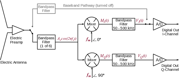
Figure C.1: Tracing a single frequency component through
the Mixers
Measuring the low frequency beats, instead of the sensor output itself,
is an engineering trade off allowing relatively low speed A/D converters to
capture spectral information far above their Nyquist frequency. Due to power
and other constraints, the fastest A/D converters on-board Waves run at 7
Msps. Thus without mixing, the highest frequency emissions for which Waves
HFRs could produce detailed spectra would be 3.5 MHz. This is insufficient
for the task at hand. Due to Jupiter's strong magnetic field, emissions
produced via the cyclotron maser instability near the Jovian poles are
expected to be well above 10 MHz. Measuring these emissions near their
source region is one of the primary tasks of the instrument.
The figure above provides a block diagram of the signal conditioning and
measurement apparatus within the Waves High Frequency Receivers. Incoming
signals either pass through the baseband pathway, which omits the mixers,
or through one of 6 band pass filters. The output of the selected filter
is split and sent to two frequency mixers. Each mixer multiplies it's input
signal by a locally synthesized pure tone, however for the lower mixer (the
Q channel) the tone is 90 degrees out of phase with the upper mixer (the I
channel). As demonstrated in equation (1), mixing in this manner produces
both low frequency beats along with much higher frequency components. To
keep from aliasing the high frequency fe + fm
components into the final sampled signal, a downstream band pass filter is
used which rolls off at less than the Nyquist frequency of the final A/D
conversion stage. In this case the high point roll-off is at 500 kHz.
Finally, both signals are sampled simultaneously at 1.3125 MHz and stored
for transmission to the ground.
Equation (1) provided the output of an ideal mixer for which a single
pure tone, Aecos(2πfet), is present on the
input. But Waves has two mixers whose local oscillator is out of phase by
90°, so for the same incident tone the ideal mixing equation for the
second mixer follows.
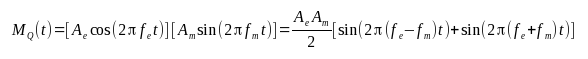
|
(2) |
As in equation (1) only the first term of the last equality matters as the
fe + fm term is filtered after mixing.
Combining (1) and (2) as a complex value, and dropping the high frequency
terms to represent the action of the downstream filters, gives the following
relationship between the mixed signal and incident pure tone.

|
(3) |
Note that unlike MI(t) and MQ(t),
V(t) is only a function of fe - fm and
time. Since only the frequency difference matters equation (3) can be
simplified by defining f to be difference between the mixer
frequency and the incoming tone. So using
f = (fe - fm) we have:
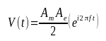
|
(4) |
The form of equation (4) is starting to look familiar. In essence, mixing
an input signal with a local oscillator and then truncating higher order
frequencies is starting to look a lot like operating on the emission
amplitudes with a Fourier kernel in fe - fm
space, instead of the traditional fe space.
The relation above is only true for an incident signal which is a pure sine
wave. This is rarely the case, however making the safe assumption that the
incident emission can be described as a superposition of pure tones of
arbitrary phase, equation (4) becomes:
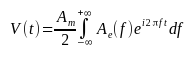
|
(5) |
where Ae(f) is a complex amplitude containing both
magnitude and phase information. Finally in this form we can see, just by
inspection, that equation (5) is the inverse Fourier transform of amplitude
components Ae(f).
In the analog world the voltage out of the band-pass filter is a continuous
function of time, however we only know these voltages at specific time
intervals, as determined by the sampling rate of the A/D converts. By the
sampling theorem we will only be able to determine the amplitude for N
discrete frequency bins, where N is the number of points collected as a
single time series by the A/D converters. So, writing (5) for discrete
sampling gives:
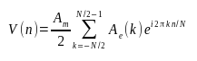
|
(6) |
where f = k fs / N and t = n / fs.
Again, by inspection, this relationship is just the inverse Discrete
Fourier Transform (DFT) of Ae(k), up to a scaling constant.
Thus the associated forward transform is:
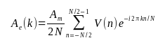
|
(7) |
Equation (7) forms the basis of how the ground software recovers spectral
information from emissions whose frequencies are above the Nyquist frequency
of the A/D converters.
Specifically, to recover the spectral information the ground software
preforms the forward transform of V(n), which is the complex vector
with components, VI(n) + iVQ(n). The
output of this transform is scaled using calibration constants for the mixer
gain to produce the vector Ae(k). Finally, frequency values
are assigned to the resulting bins via the relation:
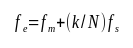
|
(8) |
