T. L. GARRARD(1), N. GEHRELS(2), and E. C. STONE(1)
1 California Institute of Technology, Pasadena, CA 91125, U.S.A
2 NASA Goddard Space Flight Center, Greenbelt, MD 20771, U.S.A.
The Heavy Ion Counter on the Galileo spacecraft will monitor energetic heavy nuclei of the elements from C to Ni, with energies from ~ 6 to ~ 200 MeV nucl-1. The instrument will provide measurements of trapped heavy ions in the Jovian magnetosphere, including those high-energy heavy ions with the potential for affecting the operation of the spacecraft electronic circuitry. We describe the instrument, which is a modified version of the Voyager CRS instrument.
The Heavy Ion Counter (HIC) is included on the Galileo spacecraft primarily for the purpose of monitoring the fluxes of energetic heavy ions in the inner Jovian magnetosphere and high-energy solar particles in the outer magnetosphere in order to characterize the ionizing radiation to which electronic circuitry is most sensitive. The measurements performed will also be of scientific interest, since the instrument's large geometry factors and extended energy range will provide spectral information for ions from 6C to 28Ni with energies of ~ 6 to >~ 200 MeV nucl-1. In this article we will concentrate on Jovian magnetospheric science. We review here previous scientific results concerning trapped high-energy heavy ions, describe anticipated new findings with Galileo, and provide a brief instrument description.
During the Voyager encounters with Jupiter, it was discovered (Krimigis et al.,1979a, b; Vogt et al., 1979a, b) that a major component of the trapped radiation in the inner Jovian magnetosphere is energetic heavy ions. The dominant heavy species inside ~ 10 RJ in the MeV nucl-1 energy range were found to be oxygen and sulfur, with sodium also present. This is illustrated in Figure 1 which compares the elemental composition between 4.9 and 5.8 RJ with the more normal solar-like composition found in the same energy range in the middle and outer magnetosphere. The abundances in the inner magnetosphere indicate that the source of the ions is the surface or atmosphere of Io.
The phase space density of the energetic oxygen and sulfur ions has a positive radial gradient (i.e., increasing outward) in the inner magnetosphere (Gehrels et al., 1981), implying that the diffusive flow at these energies is inward. On the other hand, the density of the oxygen- and sulfur-rich plasma in the inner magnetosphere is highest at the Io plasma torus and decreases outward (Siscoe et al. 1981). Barbosa et al. (1984) have proposed that charge exchange in the plasma torus produces fast neutrals which escape to the outer magnetosphere where ~ 0.2% are reionized by solar ultraviolet or electron impact and recaptured Some of the newly created ions are subsequently energized by stochastic acceleration caused by magnetohydrodynamic waves, producing ions with large magnetic moments that adiabatically diffuse inward, some attaining energies in excess of 30 MeV nucl-1 in the inner magnetosphere.
Fig. 1. Measured element (Z ) distribution for heavy ions in the Jovian environment with energies from 7 MeV nucl-1 to typically ~ 18 MeV nucl-1. (a) 4.9 to 5.8 RJ, ~ 1 hour elapsed time. (b) Outside ~ 11 RJ, 9 days elapsed time. From Vogt et al. ( 1979a). Because the measurement efficiency is independent of Z, the observed distributions directly reflect the relative abundances of the energetic nuclei in each panel.
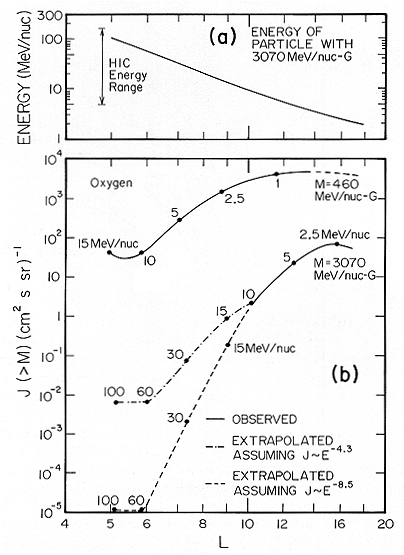
As the energetic ions flow inward, they are lost from the magnetosphere, presumably by pitch-angle scattering of the mirroring particles into the loss cone (see, e.g., Thorne, 1982). The strength of this loss mechanism determines the rate at which the heavy ions precipitate into the Jovian atmosphere, exciting ultraviolet and X-ray auroral emissions. At the time of the Voyager 1 encounter in March 1979, it appeared losses due to pitch-angle scattering were occurring at nearly the maximum rate, resulting in the precipitation of ~ 1024 ions s-1 above ~ 70 MeV nucl-1 G-1, with an extrapolation down to 10 MeV nucl-1 G-1 suggesting the possibility of a loss rate of ~ 10^26 ions s-1 and an auroral power of ~ 1013 W (Gehrels and Stone, 1983). The evidence that major losses are occurring in the magnetic moment (energy) range appropriate to HIC is shown in Figure 2, where the total inward flow rate of oxygen ions with magnetic moments greater than several thresholds is given as a function of radial distance (L) from Jupiter. The number of inflowing ions first decreases inside 15 RJ and falls off sharply inside 10 RJ.
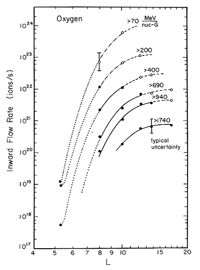
Fig. 2. The inward flow rate of oxygen ions with magnetic moments greater than the indicated values as a function of distance, L, in RJ. The filled circles are from measured spectra and the open circles from extrapolation of the spectra. Typical uncertainties in the measured and extrapolated points are dominated by uncertainties in the diffusion coefficients. There is, in addition, a factor of 3 absolute uncertainty that applies to all points. From Gehrels and Stone (1983).
The curves in Figure 2 also illustrate that only a small fraction of the trapped particles survive to produce the trapped radiation at 5 RJ. As a result, changes in the rate of pitch-angle scattering can result in significant changes in the flux of particles reaching5 RJ. It is therefore important to better characterize not only the flux at 5 RJ, but also the nature and any long-term variability in the loss mechanism operative outside of 5 RJ.
The HIC instrument should provide new information on the spectra of heavy ions at higher energies than previously possible. As illustrated in Figure 3, fluxes at these energies are based on extrapolations of spectra measured at lower energies and as a result are very uncertain.
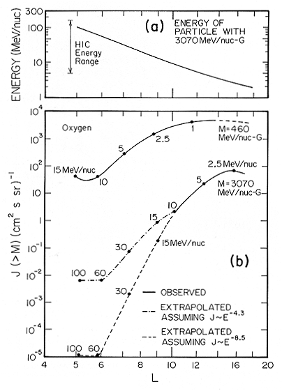
Fig. 3. (a) The energy of a particle with magnetic moment 3070 MeV nucl-1 G-1 as a function of radial position compared with the HIC energy range. (b) The integral flux of oxygen ions with magnetic moments greater than 460 MeV nucl-1 G-1 and 3070 MeV nucl-1 G-1 as functions of radial position. The solid lines represent data from the Voyager CRS instrument, and the dashed lines are possible extrapolations. The energy of the particles is indicated by the numbers at specific radial locations along the intensity curves.
Two different estimates of the expected fluxes of oxygen ions are shown in Figure 3 (b) for magnetic moments of >= 3070 MeV nucl-1 G-1 and >= 460 MeV nucl-1 G-1, corresponding to particles with E >= 100 MeV nucl-1 and >= 15 MeV nucl-1 at 5 RJ. The >= 15 MeV nucl-1 flux was directly measured by the Cosmic-Ray Science instrument (CRS) on Voyager 1 and is reasonably certain. The >= 100 MeV nucl-1 flux, however, has been determined by extrapolation, and is therefore quite uncertain as indicated by the two different profiles. The dot-dashed line is the result of an assumption that J(>E) proportional to E4.3 which is based on a least-squares fit of a power law to Voyager 1 data in the energy interval from 7 to 20 MeV nucl-1. Because of limited lifetime and geometrical factor, Voyager 1 observed no particles with energies >= 30 MeV nucl-1, so a much softer spectrum is also possible at higher energies as indicated by the dashed line corresponding to J(>E) proportional to E-8.5 These two extrapolations differ by a factor of ~ 500 in the predicted of flux of oxygen with E >= 100 MeV nucl-1 at 5 RJ.
Measurements with the HIC instrument will significantly reduce the uncertainty in the high-energy fluxes. As shown in Figure 3(a), the energy of a 3070 MeV nucl-1 G oxygen ion is within the HIC energy range into 5 RJ. The geometry factor for E > 20 MeV nucl-1 oxygen ions (inside 8.5 RJ for 3070 MeV nucl-1 G-1 ions) is ~ 4 cm2 sr compared with 0.88 cm^2 sr for the Voyager CRS instrument. More importantly, the livetime for measuring oxygen and sulfur ions with E >= 50 MeV nucl-1 will be essentially 100% because a polling priority system (see instrument description section) will discriminate against the large fluxes of protons and electrons that dominate the CRS analysis rate. As a result, a flux of only 10-5 cm-2 s-1 sr-1 should produce 1 analyzed event in 10 hours, the time that Galileo is inside 7 RJ.
Figure 3 indicates that the oxygen ions which have >= 100 MeV nucl-1 at 5 RJ have >= 10 MeV nucl-1 at 10 RJ. Thus, as Galileo makes repeated orbital passes in the vicinity of Europa, it will be possible to monitor the fluxes of particles with M >= 3000 MeV nucl-1 G-1 throughout the mission. Such long term information is especially important, since there are a number of reasons why the fluxes might vary. For example, the flux of high-energy ions could be measurably affected by changes in the density of the Io plasma torus which is the source of the escaping neutral atoms and by changes in the solar ultraviolet which re-ionizes the neutrals in the outer magnetosphere. The HIC instrument will measure any time dependence of the energetic heavy ion fluxes and permit correlative studies of any associated changes in auroral emissions or diffusion processes.
Figure 3 also illustrates that the fluxes at 5 RJ depend strongly on the loss processes occurring inside of ~ 15 RJ. It is postulated that the losses are due to pitch-angle scattering of the mirroring particles into the loss cone, and that the rate of scattering is close to the strong pitch-angle diffusion limit in the inner magnetosphere (Thorne, 1982; Gehrels and Stone, 1983). At this limit there is sufficient pitch-angle scattering to refill the loss cone as rapidly as particle precipitation empties it, resulting in a nearly isotropic pitch-angle distribution. Since the HIC detectors will view nearly perpendicular to the spacecraft spin axis, essentially complete coverage of the pitch-angle distribution will be possible. Investigation of any time dependence of the loss process will also be possible as Galileo repeatedly passes through the radial range between 15 and 10 RJ where the radial profiles in Figure 2 indicate that significant losses occur.
The Galileo Heavy Ion Counter (HIC) consists of two solid-state detector telescopes called Low Energy Telescopes or LETs. Use of these two telescopes over three energy intervals provides the geometry factor and energy range necessary to determine the fluxes of the heavy, penetrating radiation to which solid state memories are most sensitive. Heavy collimation and high discrimination thresholds on all detectors provide the necessary immunity to accidental coincidences from the large proton background. Three-parameter analysis provides additional rejection of background.
Two separate telescopes are included in order to cover a wide energy range while minimizing pulse pile-up through the optimum selection of detector and window thicknesses. The LET E is optimized for the detection of nuclei with energies as high as 200 MeV nucl-1, requiring thicker detectors. Thick windows protect this system from low-energy proton pile-up, but also exclude lower energy oxygen and sulfur nuclei. The second telescope, LET B, has a substantially thinner window so that it can detect lower energy nuclei (down to ~ 6 MeV nucl-1), especially in the outer magnetosphere. The properties of the two telescopes are indicated in Table I and discussed below.
-------------------------------------------------------------------------------
Detector            Radius             Thickness               Threshold
                     (cm)             (micro-meter)              (MeV)
-------------------------------------------------------------------------------
LB1                  0.95                 32.1                    0.3
LB2                  0.95                 29.6                    0.4
LB3                  1.13                421                      3.7
LB4                  1.13                440                      2.0
LEI                  0.95                 30.4                    9.3(1.4)*
LE2                  0.95                 33.4                    2.0(0.3)*
LE3                  1.13                463                     25(5.0)*
LE4,5                1.66              ~2000                    117(23)*
-------------------------------------------------------------------------------
*High gain.
The LET B telescope in shown in Figure 4. In this telescope ions which penetrate LB1 and LB2 and stop in the thicker LB3 detector are analyzed. Detector LB4 is used in anti-coincidence. (If desired, the command system can be used to allow analysis for ions which penetrate LB1 and stop in LB2, or for ions which stop in LB1 . Also detector LB4 can be turned off.) Lighter nuclei (especially hydrogen and helium) are rejected by 'slant' discrimination with a weighted sum of the signals from the front three detectors,
SLB = LB1 + 0.42 LB2 + 0.2 LB3
required to be above about 9.6 MeV.
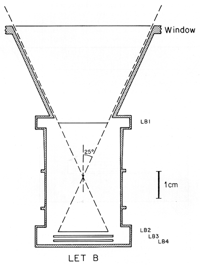
Fig. 4. Schematic cross section of the LET B telescope. The dotted housing is Al. Only the active regions of the detectors are shown.
The thin window (25 µm Kapton) shown in the figure serves for thermal control and for protection from sunlight. All detectors are surfacebarrier type. An important feature is the use of keyhole detectors for LB1 and LB2, which define the event geometry. The active area of these detectors excludes the nonuniform edge of the silicon wafer through the use of keyhole-shaped masks during the deposition of the Au and Al contacts.
This telescope is an improved version of the Voyager CRS LETs (Stone et al., 1977) which have demonstrated charge (Z) resolution of 0.1 charge units at oxygen under solar flare conditions (Cook et al., 1980) and 0.2 charge units at ~ 5 RJ, Voyager 1's deepest penetration of the Jovian magnetosphere (Gehrels, 1982). Additional collimation and the thicker window decrease the HIC LET's response to background protons in the Jovian magnetosphere. The flux of protons in detector L1, for example, should be reduced by at least a factor of 10 from that observed on Voyager 1.
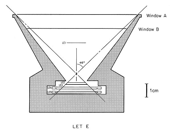
Fig. 5. Schematic cross section of the LET E telescope. The dotted housing is Al. Only the active regions of the surface-barrier detectors (LE1, 2, 3) are shown. The LiD detectors (LE4, 5) are active inside the groove on the silicon wafer. LE1 is supported by a very light-weight spider arrangement.
The higher energy LET E telescope is illustrated in Figure 5. In order to measure the flux of heavy nuclei at higher energies, LE4 and LE5 are each 2000-micro-meter lithium-drifted detectors. The front detectors, LE1, LE2, and LE3, are identical to their LET B counterparts, providing spectral continuity and overlap. The collimator housing is relatively thick to provide background immunity and has a large opening angle to provide a large geometrical factor. The windows are 76 micro-meter Kapton and 254 micro-meter Al. As in LET B, low charge (low Z) events are recognized and rejected by a slant discriminator,
SB = LE1 + 0.5 LE2 + 0.1 LE3 + 0.04(LE4 + LE5),
where SB must exceed 9.6 MeV to allow analysis.
For intermediate energies, a narrow-angle geometry is defined by LE1 and LE2 for particles stopping in either LE2 or LE3. For the highest energies, where the fluxes are exceedingly small, measurements are made with the wide-angle geometry defined by LE2, LE3, LE4, and the collimator. LEI is not required but its discriminator is recorded as a tag bit. LE5 distinguishes stopping and penetrating events. The maximum energy observed is determined by the LE2 discriminator threshold. This maximum is ~ 185 MeV nucl-1 for oxygen as noted in Table II. To allow detection of penetrating galactic cosmic-ray nuclei at higher energies in the outer magnetosphere, the LET E pre-amplifier gains can be increased by a factor of 5 to 7 by command.
With the exception of spacecraft interface circuitry, all of the electronics were originally part of the Proof Test Model of the Voyager Cosmic-Ray Science Instrument (CRS), and additional detail may be found in Stone et al. (1977) and Stilwell et al. (1979). With the adjustment of amplifier gains and discriminator thresholds and the incorporation of thicker detectors, collimators, and windows, it has been possible to develop an instrument which is optimized for the measurement of high-energy heavy ions trapped in the Jovian magnetosphere. Minor modifications to the logic allow the instrument to recognize events of the various types mentioned above, which are summarized in Table II.
Event data are stored in buffers which are read according to a polling scheme which prevents domination of the telemetry by any one type of event. The buffer polling logic cycles through the five buffers listed in Table II, reading out one each minor frame (2/3 s) and stepping to the next non-zero buffer on the subsequent minor frame. If a particular type of event occurs less than 0.3 times per second (i.e., is rare) then all of that type will be transmitted regardless of activity in other event types. If a particular type of event occurs more often than 0.3 times per second, it will be readout at least 0.3 times per second and more of ten if the other event buffers are empty.
Telemetry of counting rates and pulse height analyzed events is rapid compared to the nominal 3 rpm spin rate of the spacecraft; thus pitch-angle distributions of the trapped radiation can be measured. Both telescopes have their axes oriented near the spin plane for this purpose. The time resolution of the HIC is in the range from 2/3 to 2 s, implying an angular resolution in the range from 12° to 36°, which is to be compared to the telescope opening angles of 25° in narrow geometry mode and 46° in wide geometry mode.
Many of the functions of the coincidence logic and the buffering/readout scheme can be modified by command to optimize the instrument for changing environments or partial failures. As noted above, commands can also be used to change gain on the LET E pre-amplifiers.
----------------------------------------------------------------------------------------------

Name             Requirement                Geometry    Z range        Oxygen          Sulfur          Signals
                                            factor                     energy range    energy range    telemetered
                                            (cm2 sr)                  (MeV nucl-1)   (MeV nucl-1)
----------------------------------------------------------------------------------------------
                         ___
LETB         LB1.LB2.LB3.LB4      0.44    C to Ni    6 to 18       9 to 22   LB1,LB2,LB3
                     ___
DUBL         LE1.LE2.LE3          0.44    C to Fe   16 to 17      24 to 25   LE1,LE2
                         ___
TRPL         LE1.LE2.LE3.LE4      0.44    C to Ni   17 to 27      25 to 38   LE1,LE2,LE3
                         ___
WDSTP        LE2.LE3.LE4.LE5      4.0     C to Fe   26 to 46      37 to 70   LE2,LE3,LE4

WDPEN        LE2.LE3.LE4.LE5      4.0     C to Fe   49 to ~185    >= 70      LE2,LE3,LE4+LE5

WDPEN        LE2.LE3.LE4.LE5.HG   4.0     Li to O   49 to ~500    -          LE2,LE3,LE4+LE5
(High gain)
----------------------------------------------------------------------------------------------
A special acknowledgement is due A. W. Schardt, whose untimely death prevented his co-authorship of this paper. This project was made possible by the development of the CRS instrument under the leadership of R. E. Vogt. W. E. Althouse (Caltech) and D. E. Stilwell (GSFC) have provided invaluable engineering and programmatic support and advice. We also are pleased to acknowledge the contributions of A. C. Cummings at Caltech; M. Beasley, W. D. Davis, J. H. Trainor, and H. Trexel at GSFC: and D. R. Johnson at JPL. This work was supported by a number of NASA contracts and grants.
Barbosa, D. D., Eviatar, A., and Siscoe, G. L.: 1984, J. Geophys. Res. 89, 3789.
Cook, W. R., Stone, E. C., and Vogt, R. E.: 1980, Astrophys. J. 238, L97.
Gehrels, N.: 1982, 'Energetic Oxygen and Sulfur Ions in the Jovian Magnetosphere', CIT Ph.D. Thesis.
Gehrels, N. and Stone, E. C.: 1983, J. Geophys. Res. 88, 5537,
Gehrels, N., Stone, E. C., and Trainor, J. H.: 1981, J. Geophys. Res. 86, 8906.
Krimigis, S. M., Armstrong, T. P., Axford, W. I., Bostrom, C. O., Fan, C. Y., Gloeckler, G., Lanzerotti, L. J., Keath, E. P., Zwickl, R. D., Carbary, J. F., and Hamilton, D. C.: 1979a, Science 204, 998.
Krimigis, S. M., Armstrong, T. P., Axford, W. I., Bostrom, C. O., Fan, C. Y., Gloeckler, G., Lanzerotti, L. J., Keath, E. P., Zwickl, R. D., Carbary, J. F., and Hamilton, D. C.: 1979b, Science 206, 977.
Siscoe, G. L., Eviatar, A., Thorne, R. M., Richardson, J. D., Bagenal, F., and Sullivan, J. D.: 1981, J. Geophys. Res. 86, 8480.
Stilwell, D. E., Davis, W. D., Joyce, R. M., McDonald, F. B., Trainor, J. H., Althouse, W. E., Cummings, A. C., Garrard, T. L., Stone, E. C., and Vogt, R. E.: 1979, IEEE Trans. Nuc. Sci. NS-26, 513.
Stone, E.C., Vogt, R.E., McDonald, F.B., Teegarden, B.J., Trainor, J.H., Jokipii, J.R., and Webber, W. R.: 1977, Space Sci. Rev. 21, 355.
Thorne, R. M.: 1982, J. Geophys. Res. 87, 8105.
Vogt, R. E., Cook, W. R., Cummings, A. C., Garrard, T. L., Gehrels, N., Stone, E. C., Trainor, J. H., Schardt, A. W., Conlon, T., Lal, N., and McDonald, F. B.: 1979a, Science 204, 1003.
Vogt, R. E., Cummings, A. C., Garrard, T. L., Gehrels, N., Stone, E. C., Trainor, J. H., Schardt, A. W., Conlon, T. F., and McDonald, F. B.: 1979b, Science 206, 984.
In Phase 2a, HIC realtime data are collected by a CDS program for a period of time that depends on readout rate: 50 RIM (at 1 bps), 25 RIM (2 bps), or 10 RIM (5 bps), where 1 RIM = 91 minor frames and 1 mf = 2/3 sec. At the end of the collection period, another portion of the program compresses the data into their output format.
The output (before packet headers are added) consists of up to 375 bytes of binary data in two blocks. A dump of simulated data is attached as Appendix A. For details about packet headers, see MOS-GLL-3-310 (ECR 35559), Flight Software Requirements, Appendix, p. 5-47; and 625-610: SIS 2244-05 P2, Instrument Packet File. The present description is of the HIC data only.
The first block, of 143 bytes, contains rate data arranged in a predetermined format. There are 57 rate "words" of 2 1/2 bytes each, and 1/2 byte of filler (0x0) at block's end. The first byte of each rate word is a counter of the number of times that rate was read out. The rest of the word (1 1/2 bytes) gives the sum of the rate counts from those readouts, in log-compressed form. The compression scheme is the same as that in the SRD.
Several types of rate are subdivided, i.e., have more than one rate word in the output block. Each successive rate word within a type represents data taken in a later portion of the collection period. The 57 rate words appear in the following order:
10 words of DUBL  ("A" rates, for ten successive time divisions)
 6 words of TRPL  ("B" rates, for six successive time divisions)
 6 words of WDSTP ("C" rates, for six successive time divisions)
 6 words of WDPEN ("D" rates, for six successive time divisions)
10 words of LETB  ("E" rates, for ten successive time divisions)
 6 words of LE1   ("G" rates, for six successive time divisions)
 1 word  of LE5   ("F" rates, MUXN=10)
 1 word  of LE3   ("F" rates, MUXN=11)
 1 word  of LE4   ("F" rates, MUXN=12)
 1 word  of LE2   ("F" rates, MUXN=13)
 6 words of LB1   ("H" rates, MUXN=10, for six successive time divisions)
 1 word  of LB2   ("H" rates, MUXN=11)
 1 word  of LB3   ("H" rates, MUXN=12)
 1 word  of LB4   ("H" rates, MUXN=13)

(Slant data, from "F" and "H" rates with MUXN < 10 or MUXN > 13, are discarded.)
Thus for the longest collection period (50 RIM), we can distinguish ~5-min changes in the DUBL and LET B rates and ~9-min changes in the five rates that have six divisions each. At higher data rates (collection periods of 25 RIM or 10 RIM), the time resolution is proportionally better.
The second block, of up to 232 bytes, contains event data arranged in a flexible format. The contents of this block can vary considerably depending on the number and kind of events that were observed. Events have no time divisions.
The events are divided into fourteen types and kept, during the collection period, in fourteen different arrays. Each collection array can hold up to 20 or 32 events, depending on type. The array numbers determine the order in which events are output. Event types are distinguished in the output block not by absolute position (as are the rates) but by header words.
Each string of event information begins with a one-byte header. The first half-byte contains the event array number, i.e., the type. The second half-byte is a counter that gives the number of events in the string for that type, less one; i.e., counter = counts - 1. If no events were observed for a given type, no string is output.
Each event type has a characteristic word length, so the header also gives the length of the event string. Each type also has a characteristic meaning assigned to each bit in its word. For details, see Appendix B.
After all the output events comes an event counter array, which consists of a leading 'f' followed by six numbers of 1 1/2 bytes each. These show the total number of events counted in the collection period for each of six kinds of event: DUBL, TRPL, WDSTP, WDPEN, LETB, and null (tag word = 0).
The fourteen event types are distributed among the five non-null kinds as follows: DUBL, type 9; TRPL, types 5 and 12; WDSTP, types 1, 6, 13, and 14; WDPEN, types 7 and 8; and LETB, types 2, 3, 4, 10, and 11. Counts in this array include "caution" events, those whose caution bit in the tag word is set.
When rates are very low, all observed events are output and the event block is very short. When rates are very high, details of some events will be lost because of the limited size of the output block: 232 bytes will hold only about 60 events plus the counters.
If the event arrays are quite full, the program outputs sixteen events from each type, starting with number one, until it has no more room. For this situation, only events of types 1-5 will be output in detail; the rest will be lost, as in the Appendix A dump. Since the program outputs the first sixteen events of each type, events from the beginning of the collection period are favored ever more heavily as rates climb.
Bar = first rate counter of each series, or event type's header.
 x = filler nybble (always 0x0)

octal      data
address
         __                                                rates
0000000  8880 8988 1897 8179 8818 9881 8978 1798 8189 8818
                     __
0000024  9781 7988 18ed 7edf d7fd fd7f dfd7 fdfd 7fdf c7fc
         __                                   __
0000050  ed73 1fd7 3dfd 73df d73d fd73 dfc7 3ded 76df d77d
                                  __
0000074  fd77 dfd7 7dfd 77df c77c 8872 a977 3c98 73e9 873e
                                              __
0000120  9773 c987 3e98 73e9 773c 9873 e987 3eed 6b1f d6bd
                                  __    __    __    ___
0000144  fd6b dfd6 bdfd 6bdf c6bd 5e76 b5e6 815d 68b5 d697
         __                                   __    ___
0000170  0f85 20f8 5210 8601 0860 1086 0108 605e 6b05 d6ba
         __    x__                               __
0000214  5d6c 5012 ab9b 9c65 ab9b 9c65 ab9b 9c65 525c 66d5 events (@ 0217)
                               __
0000240  4e5c 66d5 4e5c 66d5 4e62 9cfc f652 9cfc f652 9cfc
              __                   x__                   x
0000264  f652 72fc a9af ca9a fca9 a082 bcab 5bca b5bc ab50
         __                                             __
0000310  924c 24c2 f0fb 794c 24c2 f0fb 794c 24c2 f0fb 79c2
                                       __
0000334  3185 a89d 3185 a89d 3185 a89d d217 2670 ca17 2670
                     __                               _
0000360  ca17 2670 cae2 19c3 d8a5 19c3 d8a5 19c3 d8a5 f003
                           x
0000404  0060 0c00 6001 17b0
The table below gives details of how each event type is compressed into its word. The tag word is discarded for all types but #9 since the array number gives much of the relevant information. The "maximum number of events" is the highest number that the program will put into that collection array.
A "small" event has all zeroes in the first half-byte of each of its PHA words. Other events are "big." A "caution" event is one whose caution bit (last bit of tag word) is set.
Consult the SRD, Table 6 (p.8), for detector correspondence to PHA words for the various event types.
Array  Word   Max #   Event Type              Bit source
No.    Len.   Evts.                      PHA3     PHA2     PHA1
----------------------------------------------------------------
 1      32     32   big LE1 WDSTP       top 11   top 10   top 11
 2       8     32   LET B single        --       --       top 8
 3      20     20   big LETB double     --       top 10   top 10
 4      32     20   big LETB triple     top 10   top 11   top 11
 5      32     20   big TRPL            top 10   top 11   top 11
 6      32     20   big !LE1 WDSTP      top 11   top 10   top 11
 7      20     20   LE1 WDPEN           top 10   top 10   --
 8      20     20   !LE1 WDPEN          top 10   top 10   --
 9      48     32   DUBL and "caution"  all      all      all   plus tag word
10 (a)  20     20   small LETB double   --       bot 10   bot 10
11 (b)  32     20   small LETB triple   bot 10   bot 11   bot 11
12 (c)  32     20   small TRPL          bot 10   bot 11   bot 11
13 (d)  32     20   small LE1 WDSTP     bot 11   bot 10   bot 11
14 (e)  32     20   small !LE1 WDSTP    bot 11   bot 10   bot 11
NOTE: The following pairs of event types have the same construction (there are only 9 different schemes): 1 & 6; 4 & 5; 7 & 8; 11 & 12; 13 & 14.