The Galileo Star Scanner as an Instrument for Measuring Energetic Electrons in the Jovian Environment

by

Paul Dennis Fieseler

A Thesis Presented to the FACULTY OF THE GRADUATE SCHOOL UNIVERSITY OF SOUTHERN CALIFORNIA in Partial Fulfillment of the Requirements for the Degree MASTER OF SCIENCE (AEROSPACE ENGINEERING)

December, 2000

Copyright 2000, Paul Fieseler


Acknowledgments

The author would like to acknowledge the following individuals and institutions:

Dr. Robin Evans/JPL for providing multiple Novice runs and advice, Dr. Henry Garrett/JPL for providing most of the EPD and HIC data used in the correlation study. Drs. McEntire/APL, Cohen/CalTech and Stone/JPL for making EPD and HIC data available. Dr. Ratliff/JPL for advice and access to drawings, Dan Porter of Galileo/JPL for providing star scanner temperature data, Steven Joy for assistance with the PDS file creation, Galileo Project Management and my thesis committee consisting of Drs. Gruntman, Shemansky and Muntz of USC/aerospace for advice and support in this endeavor.


Table of Contents

   
ACKNOWLEDGEMENTS   ii
 
LIST OF FIGURES   v
 
LIST OF TABLES   v
 
ABSTRACT   viii
 
1. INTRODUCTION   1
 
2. STAR SCANNER DESIGN AND OPERATION   3
 
2.1 Star Scanner Physical Overview
  3
2.1.2 Photomultiplier tube
  5
2.1.3 Lenses
  7
2.2 Operation
  7
2.2.1 Normal star scanner operation
  7
2.2.2 OSAD
  9
2.3 Complications in the Data
  9
2.3.1 The mixing of star light and radiation measurements
  9
2.3.2 Telemetry synchronization
  11
 
3. STAR SCANNER CALIBRATION   13
 
3.1 Pre-flight Calibration
  13
3.2 In-flight Calibration
  14
3.2.1 EPD and HIC correlation
  14
3.2.2 Comparison With Pioneer and Voyager data
  17
3.2.3 Divine model comparison
  20
3.2.4 Particle drift in the Io torus
  21
3.3 Shielding Analyses
  22
3.3.1 Shielding analysis #1
  22
3.3.2 Shielding analysis #2
  23
3.4 Best Estimation of Response
  27
3.5 Converting Star Scanner Counts to Flux
  27
3.5.1 Fit to EPD DC3 channel
  27
3.5.2 Fit to EPD B1 channel
  29
3.5.3 Fit to Divine model
  29
3.5.4 Best fit
  30
 
4. DATA ANALYSIS TECHNIQUES   31
 
4.1 Data Set Creation
  31
4.2 The Filtering Process
  35
4.3 PMT Gain Changes
  37
4.3.1 Aging and radiation damage
  38
4.3.2 PMT saturation
  39
4.4 Fatigue
  41
4.5 Noise and Variability
  41
4.5.1 Star light distribution
  42
4.5.2 Background radiation count distribution
  43
4.5.3 Sampling noise
  44
4.6 Attitude Errors
  45
4.7 Magnetic Effects
  46
4.8 Temperature Effects
  46
4.9 Calculational Errors
  47
4.10 Total Uncertainty
  48
 
5. USES OF STAR SCANNER DATA   50
 
5.1 Scientific Value
  50
5.1.1 The C22 Orbit
  51
5.1.2 Direct sensing of the solar environment
  53
5.1.3 Earth, Venus, Gaspra and Ida encounters
  54
5.1.4 Variable star detection
  55
5.2 Engineering Value
  55
5.3 The Future
  55
 
6. CONCLUSION   57
 
REFERENCES   58


List of Figures

Figure Page
1. Galileo's Trajectory for Orbits for the Year 2000 2
2. Galileo Co-ordinate System and Location of Star Scanner 4
3. Star Scanner Side View 5
4. Photomultiplier Tube 6
5. Intensity Variation Pattern Caused by a Non-Dark Sky for Orbit E15 10
6. Star Corruption Beat Pattern Superimposed on E14 Background Data 12
7. EPD DC3 data for E14 17
8. Pioneer 10 Data showing Absolute Omnidirectional Intensities of Electrons in Six Energy Ranges (Baker and Van Allen, 1976) 18
9. Star Scanner Raw Background Data Approaching Jupiter During JOI 19
10. Comparison of the Flux Response of Star Scanner and Divine-Garrett Model at Different Energies 21
11. Normalized Integral and Differential Electron Dose at Photomultiplier Tube 24
12. Normalized Integral and Differential Electron Dose at the Last Lens 26
13. Data Processing Flow Chart 31
14. Comparison of Raw Filtered and Compensated Data Sets for Orbit E14 35
15. Filtered Data for E14 Orbit 36
16. Distribution of Star Intensity Readings 42
17. The C22 Orbit 52


List of Tables

Table Page
1. Star Scanner Correlation Coefficients 15
2. Comparison of Divine Model and Typical Star Scanner Response 20
3. Novice and Divine Model Based Predictions of Star Scanner Sensitivity Range 26
4. Step Factors by Orbit 38
5. Example Uncertainties in the Compensated Data Set 48


Abstract

The Galileo spacecraft carries aboard it a photomultiplier tube based star scanner for the purpose of providing the spacecraft with an inertial attitude reference. This device has been subjected to the radiation environment within Jupiter's magnetosphere since 1995 and is providing measurements of the omnidirectional flux of 1.5 to 30 MeV electrons within about 12 Jupiter radii. The range of maximum sensitivity is roughly 4 to 15 MeV. The star scanner is measuring electrons in energy ranges similar to some channels of Galileo's Energetic Particles Detector (EPD) but the star scanner operates continuously thus providing a unique data set when EPD is not operating. The star scanner is generally not sensitive to pitch angle distribution. Data from this newly calibrated instrument is being made available via the Planetary Data System.


1. Introduction

The Galileo spacecraft was injected into Jovian orbit in December of 1995. As of September 2000, the spacecraft has followed a looping orbit that has brought it within the inner magnetosphere of Jupiter a total of twenty-eight times (fig. 1) approaching the planet as close as 4 Jupiter Radii (RJ) during the Jovian Orbit Insertion (JOI) event. For the purposes of providing an absolute attitude reference, the spacecraft carries a star scanner which continually sweeps the sky attempting to recognize stars. When this photomultiplier tube based device was constructed, it was feared that the Jovian radiation environment would cause scintillation, fluorescence or other effects which might simulate star light and cause the star scanner to falsely recognize stars and adversely affect spacecraft operations. An attempt was made to minimize this problem by the star scanner's design [Birnbaum et al. 1983, 1984]. Nevertheless, it has been discovered that the star scanner is providing a reproducible and quantifiable measurement of some facet of the radiation environment during each perijove pass. This thesis describes a successful attempt to determine the particle and energy range which the star scanner is detecting and to relate the star scanner's output to an actual flux in the environment.

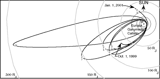
Figure 1. Galileo's Trajectory for Orbits for the Year 2000

2. Star Scanner Design and Operation

2.1 Star Scanner Physical Overview

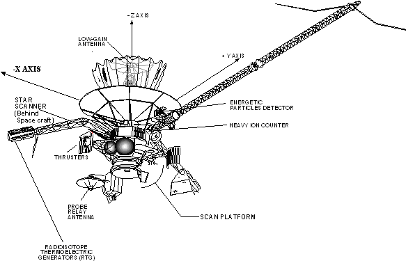
The star scanner is located on the spinning portion of the Galileo spacecraft which is referred to as the rotor. This portion of the vehicle maintains a spin rate of 0.3300 rad/sec (± .0015), thus the star scanner sweeps out 360 degrees in approximately 18.9 seconds. The instrument's boresight is aligned 80.5 degrees from the -Z axis (fig. 2) and the field of view is ± 5 degrees either side of the boresight allowing a 10 degree swath of sky to be cut.

Figure 2. Galileo Co-ordinate System and Location of Star Scanner

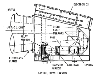
Star light enters through a baffled tube, reflects off a pair of aluminized molybdenum "right angle" mirrors, passes through two crown and one flint glass collimating lenses to a pair of slits (fig. 3). The two slits are canted at a 30 degree angle from parallel such that the focused star image passes across each slit separately producing two distinguishable pulses [Merken et al. 1993]. The separation in time of the two pulses determines the elevation (amount off the boresight along Z-axis) of the star in the star scanner's field of view. One complete rotor revolution later, the first slit again passes a pulse of light. This information is used to determine the spacecraft spin rate. Onboard algorithms use this set of data to update the spacecraft attitude quaternion.

Star light exits the slits, reflects off three more mirrors and is finally detected by a single photomultiplier tube. The folded optical path was specifically designed to prevent high energy particles from coming down the instrument's boresight and striking the glass optics or the photomultiplier tube (PMT).

Figure 3. Star Scanner Side View

There are two angle definitions in common use relative to the star scanner. The first, clock angle, is a spacecraft referenced measurement of the angle of the boresight of the star scanner as it travels a full 360 degrees with each spacecraft revolution. A clock angle of 0 degrees is in the direction opposite the +Y axis and increases in value as the spacecraft spins in a right-hand sense about the +Z axis. The second angle, termed twist, is an inertially based angle using the EME-50 coordinate system. Twist is defined as the angle between the projection of the 1950 North Celestial Pole onto the rotor's X-Y plane and the -X axis of the rotor. Twist angle increases in the opposite sense from clock such that it increases as the spacecraft spins counter-clock wise looking along the -Z axis. Since the spacecraft Z axis generally remains close to but not in the plane of the ecliptic, one degree of clock angle is only approximately equal to one degree of twist. Twist angle is much more frequently telemetered than clock; thus twist will be used when an angle measurement is needed through-out the remainder of this paper.

2.1.2 Photomultiplier tube

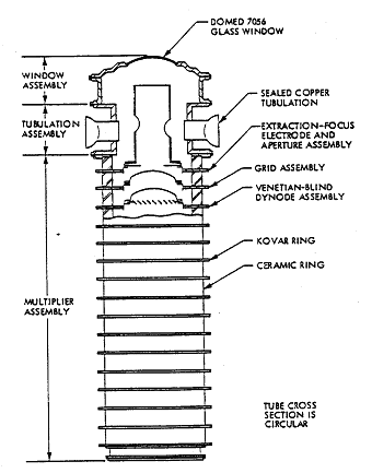
The PMTs were built by EMR Photoelectric [Birnbaum et al. 1984] starting with a 13 stage tri-alakali PMT (model # 549-01090) and modified to minimize their response to radiation. Only the "A" unit (SN #002) PMT and associated electronics have been used at Jupiter with the B-unit (SN #003) remaining un-powered. Light enters the PMT through a 0.018 mm thick domed window where it strikes a (Na)2KSb photocathode (fig. 4). The photocathode ejects electrons in response to incident photons and these electrons are amplified through a series of dynode stages to produce the output signal. Electrostatic focusing was used to reject electrons not incident from the direction of the photocathode. The main shell of the PMT is ceramic rather than glass to minimize florescence and Cerenkov effects. The star scanner operates as a photon counter with its peak efficiency at a wavelength of 410 to 430 nm. Pre-flight testing found the "A" unit PMT to have a linear response within 0.5% percent for any source up to the brightness of Sirius [Mobasser et al. 1986].

Figure 4. Photomultiplier Tube

The star scanner's PMT has no intrinsic ability to distinguish between actual light sources and apparent light sources caused by radiation effects. These apparent light sources may include direct or scattered secondary electron stimulation of the PMT photocathode or dynodes, Cerenkov or fluorescence in the three glass lenses and PMT window and Bremsstrahlung stimulation of the photocathode. Preflight calculations [Birnbaum 1983] estimated that 85% of the measured flux would be electrons directly reaching the PMT photocathode and the remaining 15% caused by Cerenkov and fluorescence in the lenses. With the flight data available, there is no way to confirm this. Despite not knowing the exact means by which the detection of the radiation operates, it is possible, as will be shown, to determine responsible particle and its flux in the environment external to the spacecraft.

Care was taken in the radiation-hardening of the PMT. An additional electrode was inserted between the photocathode and the first dynode to reject electrons over a wide range of energies that came from any direction other than the photocathode.. Also, the first two dynodes were made small to minimize any scattered or secondary electrons from being amplified as a signal. Electrons impinging on latter dynodes generally cause much less PMT signal as the fewer remaining dynodes cause less signal gain. Both theoretical and test data with 1 MeV [Birnbaum et al. 1984] electrons shows the excellent rejection of electrons of any energy incident from any direction other than directly from the photocathode A ceramic rather than glass envelope was used to prevent fluorescence and/or Cerenkov radiation from interfering. The glass in the photocathode was made extremely thin to minimize fluorescence and Cerenkov emission.

2.1.3 Lenses

Away from the PMT but in the optical path are three lenses which, when irradiated, will emit fluorescence and/or Cerenkov photons indistinguishable in the data from star light or electrons striking the PMT. These lenses are two crown glasses surrounding a lens of flint glass. Specifically, the first lens in the optical train is of Schott SK16, the middle lens of Ohara SF2 and the final, and by far least shielded lens is Ohara SK18, Melt N2 03816, Anneal type B1.

2.2 Operation

2.2.1 Normal star scanner operation

At an arbitrary part of the sky, not necessarily pointed at a star, the star scanner integrates the PMT signal coming through both slits for a 3.2 millisecond "sample". There are always four overlapping samples being taken simultaneously which have start times staggered in 0.8 msec intervals. After each sample completes, regardless of whether a specific star has been sighted, the integrated intensity value is added to a buffer containing the previous 31 samples. From this buffer, an average is created and stored on-board as a value termed "raw background radiation count" or just "background count". There is also a parameter termed "ideal background radiation count" which is used in on-board calculations but does not come down in telemetry.

At various points during the mission, a "star set" of from 2 to 6 stars are loaded into spacecraft memory containing the expected intensity and clock position of each star. When a star (not necessarily one in the star set) comes into the field of view, the star scanner electronics first determine if its intensity is above a minimum threshold determined by a combination of ground commands and autonomous adjustments on board. If the test is passed, then the intensity of this "candidate star" is held in a buffer along with the slit crossing time and the most recently calculated background count. Subsequent star intensity samples are gathered and compared to the previous intensity. The larger intensity along with its associated time and background values are returned to the buffer. When the intensity of a sample drops to half of this buffered maximum, the star scanner electronics interpret this event as an indication that the trailing edge of a star has passed the slit. At this time, the candidate star's maximum star intensity, slit crossing time and the background count value are made accessible for packetization in telemetry. As most downlink packets are thrown away due to Galileo's low bit rate capability, this star data is usually only sent to flight controllers once per several spacecraft revolutions. The data is also used by onboard algorithms to determine if the candidate star is in fact one of the desired stars in the star set. If so, spacecraft attitude information is extracted.

It is important to note that, with this scheme, the raw background radiation count is actually a combination of two things. First, prior to a given star being seen, the PMT is integrating all the light coming through both slits which include such things as light from dim stars, zodiacal light, nebula, etc. - in addition to any effects the radiation has on the PMT in that same interval. Hence, raw background radiation counts are partly a measure of whatever stray light sources are in the sky. Fortunately, this is deterministic and can usually be subtracted out.

Second, as a star is recognized, the integration of background count is continuing and so the candidate star's intensity is added in. This effect is only sometimes and partially amenable to removal. Both problems will be discussed in section 2.3.

Finally, it is important to note that since the star scanner only reports the background count upon seeing a star, the radiation data is only reported from fairly specific angles of the sky. This severely constrains any information on pitch angle distribution to a few angles.

2.2.2 OSAD

There is a second mode of operating the star scanner which is termed "OSAD" for One Star Attitude Determination. This mode is used when the radiation environment is expected to be harsh. It differs from the normal mode described above in that only one especially bright star is loaded into memory multiple times to constitute a star set. As the star is bright, it tends to have a proportionally large contribution to the background count. OSAD was used in parts of the JOI period as well as orbits C22 and later. Note that the orbit nomenclature is such that the first letter represents the Jovian moon most closely approached and the number is a sequential counter. For example, C22 means the 22nd orbit of Jupiter in which Callisto happened to be the satellite most closely approached. When "J" is used for the letter, then no moon was particularly targeted and the "J" simply means Jupiter.

2.3 Complications in the Data

2.3.1 The mixing of star light and radiation measurements

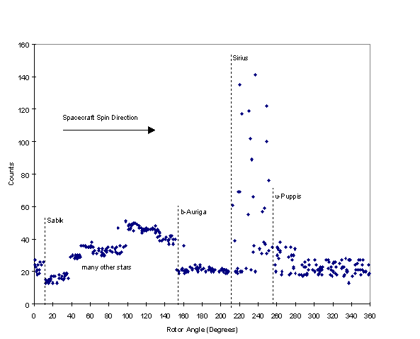
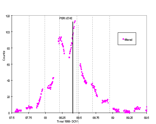
After each star sighting, no additional background count is made available in telemetry until the next candidate star is recognized. In an environment far from the radiation belts, this scheme creates a pattern which varies as a function of rotor twist angle (spacecraft spin). This is shown in figure 5 with raw background radiation counts as the dependent variable. It can be seen that the counts rise and fall with the recognition of individual stars depending upon what the background brightness of the sky is at that point. The fact that this "star corruption" pattern is repeatable allows

Figure 5. Intensity Variation Pattern Caused by a Non-Dark Sky for Orbit E15

the creation of an algorithm to subtract out these light sources. This algorithm is performed on the telemetered data, not onboard the spacecraft. The star corruption pattern changes when spacecraft attitude is altered, either intentionally to keep Galileo's antenna pointed toward earth or incidentally, as a result of a trajectory update maneuver.

As is shown in figure 5, the bottom level of the background count at any given rotor angle and when taken outside of a radiation environment, is determined by only the brightness of the sky in proximity to a given star. Stars embedded in the brightest portion of the Milky Way reach over 50 counts. For example, the star Sabik is in a fairly dim part of the heavens but rising counts are seen soon after it as the star scanner field of view sweeps into the Northern Hemisphere portion of the Milky Way. This effect is predictable, repeats from orbit to orbit and can be reliably subtracted out. The variation or noise in background count above the bottom level is directly proportional to a given star's intensity. This is because the some, all or none of the star light may be captured in the final integration sample and then sent to the background count buffer to be averaged. For example, Sirius with an intensity of 4200 counts shows a variation of about 130 counts which is the star's intensity divided by 32. Unfortunately, the rotation of the spacecraft is generally not an integral multiple of the 0.8 msec sample rate, thus it cannot be predicted how much of a star's pulse is in any particular sample. This means that this variation cannot be subtracted out. Generally, it is a small effect which can be treated as a small source of additional noise (section 4.5.3). For the very brightest stars the best that can be done is to throw out the radiation data from the part of the sky associated with the star. This is done in the filtered and compensated data sets for stars with an intensity of >650 counts which corresponds to an uncertainty of >20 counts in the radiation data. There are only 14 stars in the sky that appear brighter to the star scanner than 650 counts.

2.3.2 Telemetry synchronization

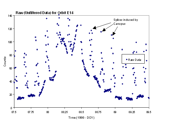
Galileo engineering data has two normal rates: 2 bps and 10 bps with the higher rates of 40 or 1200 bps used only infrequently. The star scanner data is only a portion of the total engineering data stream. Each star scanner data sample (star intensity, slit crossing time and raw background radiation count) is seen only once per 400 seconds, 80 seconds, 20 seconds or 0.667 seconds, respectively. Particularly at the 2 bps engineering rate, a beat pattern develops between the data and the spacecraft spin. At the ideal spacecraft spin rate of 0.3300 rad/sec, the spacecraft turns almost exactly 21 times for each star scanner data sample. Consequently, the star scanner reports almost the same point in the sky repeatedly with only a slow drift in twist angle. In some instances, it can take many hours before the drift completes one full revolution. There is then a spacecraft spin-rate dependent beat pattern in the background count as subsequent areas of the sky of differing brightness are measured. The situation is similar, although more complex, for the 10 bps engineering rate in

Figure 6. Star Corruption Beat Pattern Superimposed on E14 Background Data

which the spacecraft nominally turns 4.2 times for each sample. In this situation, every fifth data point is sampling nearly the same region of sky. Raw background radiation data at 2 bps is shown in figure 6 for the perijove period of orbit E14 and clearly shows the repeating spikes caused by the effect of the particularly bright star, Canopus.

3. Star Scanner Calibration

Due to their ability to penetrate significant amounts of shielding and their relatively high fluxes in the Jovian environment, high energy electrons were the immediate suspect for the cause of the star scanner's radiation response although other possibilities were considered. X-rays and gamma-rays coming from the environment external to the spacecraft would certainly be able to penetrate to the star scanner. However, these photons are not expected to dramatically increase along the magnetic equator (plasma sheet) nor drop off at Io's L-shell, and the star scanner has recorded both effects quite strongly and reliably. Thus, it is not believed that these photons are responsible for the star scanner's response. Neutrons are not expected to dominate in this environment nor remain trapped along the magnetic equator. Barring more exotic particles, only protons, ions and electrons remained for further investigation.

3.1 Pre-flight Calibration

Before launch, considerable effort [Birnbaum et al. 1984] was expended to reduce the effects of the Jovian radiation environment on the star scanner's detection of star light. As part of this testing, an unshielded PMT of the same design as those on the spacecraft was probed with Cobalt 60 which is a source of up to 1.33 MeV gamma rays and ~ 1 MeV electrons. The purpose of this work was to verify that the specially modified PMT has a muffled response to the radiation as compared to the off-the-shelf model. Although the results were as expected, the PMT was still found to respond to high-energy electrons despite the radiation-hardening (see section 2.1.2).

This is the only pre-flight radiation calibration of the star scanner or its components. There is insufficient data to quantitatively relate the results of this test to the shielded PMT's response in actual operation.

Protons or ions would not directly stimulate the PMT photocathode or anode, nor would they directly cause Cerenkov or fluorescence. Nevertheless. these particles could still kick-off secondary electrons that might be responsible for the star scanner's response. Thus, although pre-flight testing cannot distinguish which particle is causing the background signal, it is at least consistent with electrons coming directly from the environment.

3.2 In-flight Calibration

An attempt was made to correlate the star scanner curves with data from calibrated instruments aboard Galileo. These included the Heavy Ion Counter (HIC) and the Energetic Particles Detector (EPD) which together cover a range of protons from 20 KeV to 55 MeV, ions from 10 KeV/nucl to 200 MeV/nucl and electrons from 15KeV to > 11MeV [Garrard et al. 1992, Williams et al. 1992]. Data sets from Pioneer 10 and 11 as well as Voyager 1 [Van Allen 1976, McDonald et al. 1976, Fillius 1976, Schardt et al. 1983] were also consulted. The EPI instrument aboard the Galileo Probe only gathered two data points in a region which overlaps that seen by the star scanner and was not used in this study. Ulysses data was consulted (section 5.1.1) but was not used for star scanner calibration due to the great differences in trajectories between that spacecraft and Galileo.

3.2.1 EPD and HIC correlation

For the purposes of correlating the star scanner data with other calibrated scientific instruments aboard Galileo, a file containing HIC, EPD and star scanner data was created [Garrett and Evans 2000] which binned the data into ten minute periods. The data was reduced such that a single data point represented the average of a channel's counts over each ten minute interval. This data was then read into Microsoft Excel such that each column represented a different channel. The correlation between star scanner data and each channel of EPD and HIC was studied. Table 1 lists

Table 1 - Star Scanner Correlation Coefficients

Physical C20C21C22I24E26Ave.
RJ Radial Distance from Jupiter -0.84-0.57 -0.80 -0.73 -0.95-0.78
WLONG West Long. of the s/c in Sys III - degrees 0.02-0.18 0.13 0.38 0.34 0.14
LAT Latitude of the s/c in degrees - North is + -0.23-0.05 0.20 0.06 -0.60-0.12
BS(VIP4)Magnetic Field Model at s/c (VIP4 model) 0.95 0.94 0.91 0.95 0.95 0.94
BX(VIP4)X component of BSC -0.33-0.53 0.11 -0.69 -0.47-0.38
BY(VIP4)Y component of BSC 0.35 0.54 0.13 0.00 0.20 0.24
BZ(VIP4)Z component of BSC -0.94-0.93 -0.93 -0.94 -0.95-0.94
L(VIP4) Magnetic L shell value -0.80 0.26 -0.60 -0.03 0.98-0.04
LATM Magnetic latitude (offset tilted diplole) 0.22-0.06 0.24 -0.09 -0.03 0.06
B(DP) Magnetic Field at s/c (Offset Tilted Dipole) 0.93 0.92 0.93 0.91 0.95 0.93
L(DP) Magnetic L value -0.85-0.57 -0.79 -0.74 -0.95-0.78
EPD
E2 42 to 55 keV electrons -0.58 -0.22 0.05 -0.15 0.57 -0.07
F1 174 to 304 keV electrons -0.23 -0.07 0.35 -0.21 0.96 0.16
F2 304 to 527 keV electrons 0.02 -0.00 0.37 0.01 0.98 0.28
F3 527 to 884 keV electrons 0.70 0.39 0.63 0.63 0.99 0.67
B0 3.2 to 10.1 MeV protons, Z=1 0.91 0.83 0.91 0.97 0.52 0.83
B1 1.5 to 10.5 MeV electrons 0.97 0.94 0.97 0.97 0.99 0.97
B2 16 to 100 MeV ions, Z=2 0.82 0.62 0.82 0.78 0.59 0.73
DC0 14.5 to 33.5 MeV ions, Z=>1 0.93 0.83 0.92 0.97 0.75 0.88
DC1 51 to 59 MeV ions, Z=>1 0.98 0.99 0.98 0.99 0.99 0.99
DC2 > ~2 MeV electrons 0.91 0.83 0.92 0.92 0.93 0.90
DC3 > ~11 MeV electrons 0.98 0.99 0.98 0.99 0.99 0.99
HIC
LETB 4.8 to 17.5 MeV/Nucl 0.11 0.30 0.18 0.37 0.49 0.29
DUBL 17.0 to 18.0 MeV/Nucl 0.05 0.21 0.07 0.30 0.44 0.21
TRPL 18.0 to 24.0 MeV/Nucl 0.56 0.66 0.77 0.82 0.53 0.67
WDSTP30.0 to 48.0 MeV/Nucl 0.34 0.36 0.79 0.56 0.57 0.52
WDPEN30.0 to 48.0 MeV/Nucl -0.54 -0.47 -0.15 -0.08 -0.19 -0.29
LE1 15.1 to 25.3 MeV/Nucl 0.22 0.63 0.29 0.57 0.57 0.45
LB1 1.9 - 5000 MeV/Nucl 0.61 0.57 0.33 0.47 0.71 0.54
LB2 1.9 to 7000 MeV/Nucl 0.05 0.21 0.07 0.30 0.44 0.21
LB3 2.1 to 13000 MeV/Nucl 0.11 0.30 0.18 0.37 0.49 0.29
LB4 16.6 to 95000 MeV/Nucl 0.12 0.33 0.20 0.05 -0.04 0.13
LE2 14.9 to 176.0 MeV/Nucl 0.17 0.32 0.27 0.30 0.30 0.27
LE3 15.4 to 192.0 MeV/Nucl 0.17 0.26 0.18 0.04 0.33 0.19
LE4 17.9 to 177.0 MeV/Nucl -0.15 -0.22 0.16 -0.02 0.30 0.01
LE5 44.8 to 185.0 MeV/Nucl -0.22 -0.25 -0.20 -0.09 -0.28 -0.21

the various channels and the correlation coefficient, ρ, for five different encounters. Bold face text represents correlation above 0.9 or anti-correlations below -0.9. The correlation coefficient is the standard one such that,

where x and y stand for a particular value being sampled, μ is the mean σ is the standard deviation of either of the compared data sets.

The use of the correlation coefficient assumes that all compared data sets are normally distributed [Dixon and Massey, 1957]. This is known to be only approximately true for star scanner data but the use of the correlation coefficient provided numbers that were intuitive.

Correlations were done on five orbits, each with at least 100 different time intervals where the data were compared. Three channels consistently stand out as being well correlated, the DC3, DC 1 and B1 channels representing >11 MeV electrons, 51 to 59 MeV ions and 1.5 to 10.5 MeV electrons, respectively. Other channels which showed high values of ρ were DC0, B0 and DC2 representing 14.5 to 33.5 MeV ions, 3.2 to 10.1 MeV Protons and >2 MeV electrons.

Care must be exercised in the use of these values however. First, it is known [McEntire 2000] that the EPD proton and ion channels are contaminated by the high energy electrons; that is, the proton and ion channels are actually sensing electrons in the DC3 range. The star scanner data is not as highly correlated with the proton and ion channels such as DC1 as it would first appear. Note that the ion channels on HIC show much lower correlation coefficients for similar sorts of energies.

Turning to the electrons, it appears that the best fit is with the DC3 (>11 MeV) and then B1 (1.5 to 11.5 MeV) channels and a weakening correlation is found with decreasing energies. Keeping in mind that the quantity of electrons in the environment decreases sharply with increasing energy, it is probably true that the bulk of the B1 channel electrons are distributed towards the lower part of the 1.5 to 11.5 MeV range. The best that one can conclude here is that the star scanner is probably most sensitive to electrons somewhere in the range from 1.5 MeV to something over 11 MeV.

Figure 7 shows a plot of the EPD DC3 channel over the same time period as star scanner data is plotted in figure 5 and figure 15. Properly scaled, the star scanner data overlays the EPD data indicating the excellent fit between these two channels.

Figure 7. EPD DC3 and Star Scanner data for E14

Not surprisingly, high positive and negative correlations were also found in comparing some of the star scanner data with the physical parameters of the orbit such as the magnetic field strength and distance from Jupiter.

Figure 8. Pioneer 10 Data showing Absolute Omnidirectional Intensities of Electrons In Six Energy Ranges (Baker and Van Allen, 1976, with permission of Univ. of Arizona Press)

Finally, it is noted that the correlations in the E26 data stand out as somewhat different from the previous orbits. The only available EPD data from this orbit was in the diminished flux near the Io L-shell. It is suspected that this is reflects a difference in the distribution of the population with a given energy (change in spectrum) in this region. This is fertile ground for future study and also for further optimization of the EPD-star scanner correlation but it will not be treated further here.

Figure 9. Star Scanner Raw Background Data Approaching Jupiter During JOI

3.2.2 Comparison with Pioneer and Voyager data

A qualitative comparison was performed between star scanner and data from Pioneer 10 and Pioneer 11 [Van Allen 1979, Fillius 1976] which passed Jupiter in 1974 and 1975, respectively. This data includes protons from 200 KeV to > 80 MeV, ions to < 3 to > 500 MeV/nucl and electrons from 50 KeV to >35 MeV. Figure 8 shows Pioneer 10 data at Jupiter. A striking feature of that data set is a prominent dip in electron flux at the Io L-shell [9,7] for some channels. This dip is only noticeable for electrons < 21 MeV. The star scanner has seen this same dip in all four passes of Io and the characteristics of the dip the match Pioneer's 5 MeV channel best. See figure 9 for a comparison. Pioneer 11 shows a similar effect.

It should be noted that a pronounced flux decrease at Io is also seen with high energy protons in both Pioneer and Voyager 1. However, none of these match the star scanner profiles particularly well at other distances from Jupiter. For example, Voyager (GSFC/UNH) experiment [Schardt et al. 1983] recording 14.8 to 21.2 MeV protons seems to qualitatively match the star scanner data near Io, but the clear dip seen near Europa's L-shell is never seen in Galileo data unless the spacecraft passes within a few radii of the moon itself.

Table 2 - Comparison of Divine Model and Typical Star Scanner Response

Distance from Jupiter11 RJ9 RJ7 RJ5 RJ
Divine Model - 1 MeV flux6.4 x 1073.4 x 1072.1 x 1074.3 x 107
Divine Model - 10 MeV flux1.0 x 1057.3 x 1051.5 x 1063.7 x 106
Divine Model - 20 MeV flux1.3 x 1048.5 x 1042.5 x 1059.9 x 105
Divine Model - 30 MeV flux3.7 x 1031.7 x 1045.5 x 1043.2 x 105
Star scanner typical counts25703601500

3.2.3 Divine model comparison

Electron fluxes as predicted by the Divine model [Divine and Garrett 1983] were found at several different Jovicentric distances for four integral energy ranges. The Divine model was based on Voyager and Pioneer data. The star scanner "typical values" were selected from orbits E26 and JOI away from plasma sheet crossings at the same distances. Below, a comparison in the change in electron flux with Jovicentric distance is made between the star scanner data and that predicted by the model. Note that the increase of star scanner counts with RJ follow both the 10, 20 and 30 MeV models well. This can be better seen in figure 10 in which the flux for the model (dotted lines) and the star scanner (solid line) has been normalized at 5 RJ.

Figure 10. Comparison of the Flux Response of Star Scanner and Divine Model at Different Energies

3.2.4 Particle drift in the Io torus

An independent analysis made use of longitudinal asymmetries in the star scanner's measurements of the Io Torus. This work [Russell et al. 2000] is being submitted for publication concurrently with this thesis. The argument holds that for asymmetries to remain in the torus, the particles must be moving only slowly with respect to Io. Electrons in the 10 to 15 MeV range fit this the best. Ions of any energy would move in a direction opposite that of Io and quickly erase any asymmetries in a fashion not consistent with the star scanner's response.

3.3 Shielding Analyses

3.3.1 Shielding analysis #1

An analysis of the star scanner's shielding over 4p steradian has been done to determine the minimum energy particle that is accessible to the star scanner's internal components. There are two possible sources of the radiation induced signal in the star scanner - the PMT and the glass lenses. While in general these areas were found to be shielded to greater than 5 g/cm2, there are a few "sneak paths" where the shielding is significantly less . An analysis [Fieseler 2000] was performed which found the minimum shielding to the PMT was 3 g/cm2 over ~20% of a unit sphere which allows >4 MeV electrons to penetrate [Hastings and Garrett 1996, Price 1957].

Shielding over the last of the three lenses in the optical train was found to be a minimum of 3 g/cm2 over an area of 40% of a unit sphere allowing >4 MeV electrons to reach the glass. Although these sneak paths are somewhat small, the rapid increase of flux with decreasing energy still makes these areas the dominant source of the measured electron flux. It is not known how much fluorescence and Cerenkov light the lens will produce under such bombardment. Regardless, since the minimum shielding is approximately the same, the this analysis would conclude that the star scanner is not sensing environmental electrons below ~ 4 MeV and is probably predominantly measuring electrons in the range of 4 to 10 MeV. It should be noted that the other two lenses were found to be better shielded by 2.2 and 5 times so their contribution is ignored.

A review of Galileo documentation provides support for the above shielding analysis. The star scanner's design specifications [Bunker 1981] demand at least 5 g/cm2 of shielding. This would stop electrons less energetic than ~8 MeV and protons less than ~100 MeV [Hastings and Garrett 1996, Price 1957]. Apparently, however, the design specifications were not met in all directions.

It is also noted here that the sneak path to the PMT is somewhat directional. This might lead one to hope to be able to derive information on the pitch angle of the electrons in the environment. At the highest fluxes, there does seem to a hint of this in the data but, as explained in sections 2.2.1 and 5.1, it is not terribly useful. The sneak path to the final lens faces a much different direction. Also, the scattering and spreading of electrons and Bremsstrahlung X-rays inside the star scanner housing will tend to dilute any pitch angle information.

3.3.2 Shielding analysis #2

A second analysis was conducted using the commercially available code Novice [Jordan 1997]. The author provided a geometric model of the shielding around both the lenses and the PMT. The Divine model of the Jovian environment was used to provide flux estimations for protons and electrons along the orbital trajectory proposed for I33 which is very similar to I24 and I25. Novice uses these two inputs in a 3-dimensional Monte-Carlo analysis to estimate the flux of initial particles, secondaries and Bremsstrahlung photons at any point within the shielding. It can provide a total dose estimate at any point. The operation of the code was kindly provided by Dr. Robin Evans of JPL.

It was desired to use the output to determine what energy of electrons the star scanner is most sensitive to. This was accomplished by repeated runs of Novice, each with a different cutoff point in the Divine model. For instance, one run included electrons below 0.5 MeV. This showed virtually no particles reach the photomultiplier tube as expected. The subsequent run cut off at 1.58 MeV where there is a small increase. Subsequent steps increase logarithmically at 2.51, 3.98, 10, 20, 31.6, 50 and 100 MeV. The results are shown in figures 11 and 12. As expected, the lowest and highest energies play little role. Data for both the PMT and the most exposed lens are shown and differ little. The sneak path where shielding is at a minimum was found to be a larger area for the lens and it is believed that this explains the quicker rise of the curve in figure 12. Although it has not been determined what fraction of the background signal comes from the lens and what comes from

Figure 11. Normalized Integral and Differential Electron Dose at Photomultiplier Tube

the PMT, it is apparent that >80% of what the star scanner is sensing is between 1.58 and 30 MeV. The differential curve for both lens and PMT shows that more than 40% of the signal comes from electrons in the 1.58 to 2.51 MeV bin indicating that this is the energy range that the star scanner is most sensitive to. This is a little lower energy than expected based on the previous and following analyses. It is believed that the difference is caused by the fact that the Novice code is more comprehensive when considering things like Bremsstrahlung which can penetrate better than an electron from which it was created.

Figure 12. Normalized Integral and Differential Electron Dose at the Last Lens

Uncertainties between the two shielding models may also play a role. Finally, it is noted that neither shielding analysis was so exhaustive as to consider every bolt, circuit board and bracket. The models represent the minimum shielding material, thus both models under-estimate by a slight but unknown amount the energy of particles able to penetrate the PMT and lenses.

Table 3 - Novice and Divine Model Based Predictions of Star Scanner Sensitivity Range

For PMT
Thickness (mils)2505111040213043508870
Proportional area (percent)0.010.014.6741.7253.550.04
Min. Energy (MeV)3.56.41325100500
Divine Model Flux (particles/cm2 sec) 5 RJ1.3E+075.0E+061.9E+067.0E+055.8E+020.0E+00
7 RJ5.0E+062.5E+061.5E+062.0E+054.2E+020.0E+00
9 RJ1.2E+074.0E+065.9E+055.0E+049.6E+010.0E+00
11 RJ1.4E+073.5E+061.2E+051.2E+041.3E+020.0E+00
Percent Effectiveness (flux * area) at 5 RJ0.230.0916.0583.540.090.00
at 7 RJ0.170.0741.9557.560.160.00
at 9 RJ1.690.7253.4044.080.110.00
at 11 RJ9.162.9543.9943.300.610.00

For Last Lens
Thickness (mils)241481959191038207630
Proportional area (percent)0.01010.0845.9343.530.45
Min. Energy (MeV)3.56.4132580300
Divine Model Flux (particles/cm2 sec) at 5 RJ1.3E+075.0E+061.9E+067.0E+058.0E+030.0E+00
at 7 RJ5.0E+062.5E+061.5E+062.0E+054.0E+030.0E+00
at 9 RJ1.2E+074.0E+065.9E+055.0E+041.0E+030.0E+00
at 11 RJ1.4E+073.5E+061.2E+051.2E+046.0E+020.0E+00
Percent Effectiveness (flux * area) at 5 RJ0.250.0036.9962.090.670.00
at 7 RJ0.200.0061.6437.450.710.00
at 9 RJ1.430.0070.7427.320.520.00
at 11 RJ7.270.0062.7828.601.360.00

Novice also gives its estimate of the shielding thickness as a function of area, similar to the crude hand analysis attempted in the first shielding analysis. These results are presented in table 3 for both the PMT and the lens. This table was produced in several steps. First, the Novice output of the shielding thickness was measured along paths from random directions outside the star scanner to the PMT head or last lens. This was part of the Monte Carlo analysis with a total of 45,625 and 46,453 ray tracings used, respectively. Novice also produced an area estimate of the fraction of the surrounding 4p steradians at each shielding thickness. This shielding was conservatively assumed to be aluminum and was then equated to a minimum energy electron that could directly penetrate the aluminum [Hastings and Garrett 1996, Price 1957]. At a given energy the Divine model was used to determine the integral omnidirectional flux of electrons at the given energy for four distances from Jupiter. The final columns in the table are a normalization of the star scanner response (predicted flux and area). This shows that, to a first order, there is no response until at least 3.5 MeV with the star scanner remaining sensitive to > 25 MeV.

This table's last column also hints that the star scanner response is dependent upon Jovian distance due to a softening of the spectrum. For example, see the change from 0.23% to 9.16% for the case with 250 mils (0.635 cm) of shielding. While this RJ dependency is probably a real reflection of the star scanner's response to the environment, the effect is not overwhelming, the star scanner generally cannot measure beyond 12 RJ anyway and it is known that the Divine model does not model the hardening of the spectrum, especially in the vicinity of Io, with enough fidelity to attempt to further calibrate the star scanner.

3.4 Best Estimation of Response

Considering all of the above factors, there is no single energy which can be identified as being the one the star scanner responds to the best. It can only be stated that the star scanner appears to be sensing electrons predominantly in the range of 1.5 to 30 MeV with a maximum sensitivity probably around 4 to 15 MeV.

3.5 Converting Star Scanner Counts to Flux

3.5.1 Fit to EPD DC3 channel

Making use of EPD's measurement of electron flux in the environment, a scaling equation can be created for changing star scanner "counts" to an actual flux of electrons in electrons cm-2 sec-1. After comparing multiple orbits, it was found that the relationship between star scanner counts and EPD counts was not steady but instead varied approximately linearly with Jovicentric distance. For DC3, the following power law gives a reasonable (within factor of 2) fit to relate EPD counts to star scanner counts.

EPD counts = [(58.642 * (RJ1.1208)] * CC             {2}

where CC, compensated counts, is star scanner background count data corrected for a variety of systematic errors (section 4.1).

The number in brackets varies from about 277 at 4 RJ to 950 at 12 RJ. Once star scanner counts have been put on an EPD-equivalent basis, then they are multiplied by 29.92 which is a conversion supplied [McEntire 2000] to change EPD counts to omnidirectional, integral electrons cm-2 sec-1. The final equation then is:

Flux (#electrons cm-2 sec-1) = 29.92 * [(58.642 * (RJ1.1208)] * CC             {3}

As a crude, independent check, it was predicted [Ratliff 1993] based on environmental models [Divine and Garrett 1983] at 4 Jupiter radii that a flux of 1.0 x 10⁸ electrons/cm-2 s-1(>3 MeV) would be incident upon the spacecraft which corresponds to ~12,050 counts by the above scaling factor. The actual raw star scanner data at 4 RJ was 5200 counts but the compensated (adjusted for saturation) was found to be 11,300 counts. It should be noted that the above flux estimate is certainly no more accurate than a factor of two as it depends on EPD data of unknown precision and accuracy, the Divine model which advertises accuracy only to a factor of two, and the assumption that the DC3 channel is a good match for the star scanner.

3.5.2 Fit to EPD B1 channel

The same procedure as above was done for the B1 channel. The EPD conversion factor for this channel was 166.7. The final equation was found to be:

Flux (#electrons cm-2 sec-1) = 166.7 * [(1.4574 * (RJ 1.9039)] * CC             {4}

Thus the flux is about 29,400 counts at 4 RJ probably indicating that this B1 channel starting at 1.5 MeV is seeing a larger flux than the star scanner. This is consistent with the belief that the star scanner is sensitive to higher values since the flux of electrons drops off with increasing energy.

3.5.3 Fit to Divine model

To avoid the reliance on EPD, the same technique was applied to fit the predictions of for integral 10 and 5 MeV electrons of the Divine model. In this case, the equation to convert star scanner counts was

Flux 10 MeV (#electrons cm-2 sec-1) = [60.087 RJ 2.181] * CC             {5}

Flux 5 MeV (#electrons cm-2 sec-1) = [0.0612 RJ 5.9101] * CC             {6}

Using the Divine model integral flux at 4 RJ, this would predict roughly 3,150 counts for 10 MeV, a factor of three low. Repeating for 5 MeV gives 37,500, a factor of three high. It was also noted that the curve for the star scanner data fit very well with the model predictions with a correlation of 0.99.

3.5.4 Best fit

The DC3 fit of equation 3 seems to give the best overall result although it is probably no more accurate than somewhere between a factor of 2 to 5.

4. Data Analysis Techniques

4.1 Data Set Creation

Figure 13 - Data Processing Flow Chart

The originally telemetered raw background data went through a set procedure to create the final compensated data set. This process is illustrated schematically in figure 13 and the details are described in the remainder of Section 4.

The ultimate goal of this work was to create a publicly accessible star scanner data set that was as corrected for systematic errors as possible and identifies the remaining errors. This is termed the "compensated data set" and is being made available via the Planetary Data System (PDS). Each compensated data set created includes the following information:

Each encounter is kept as a separate data file. Additionally, at the discretion of the PDS, each file may be expanded to include radial distance from Jupiter, L distance, System III latitude and longitude and magnetic latitude. If not, these are currently available as separate files in the PDS.

In the above list, the first five parameters were queried from the Galileo mission data archive. The thrusting event closest to and prior to the encounter was identified. Starting after the completion of this activity until about 18 RJ before the encounter, a period of data was isolated as a baseline where the star scanner response was still unaffected by radiation. Raw background count data from this period was parsed by twist angle and plotted. From this, the star corruption pattern (section 2.3) could be extracted and subtracted. Occasionally, due to the close proximity of a thrusting event and the encounter, a baseline period starting at least 15 RJ after the encounter was chosen.

Immediately after querying the data, the data set was listed in Excel in time order. During the encounter period, the raw background counts and twist angle were retrieved. As the star scanner's perception of light itself is a function of the radiation it is seeing, the star corruption pattern could not be directly subtracted from all the data at this point. Thus, the value to be subtracted at each angle was first converted to the ideal or non-saturated system (see section 4.3.2) assuming zero radiation and then re-converted to the real world standard using the current raw radiation count. This lowered the value of the subtractant an amount appropriate to the radiation conditions. The filtered data set was then produced by subtracting this new number from the original raw background.

An intermediate or "adjusted" data set was created to account for the degradation in star scanner gain over time (section 4.3.1). At this point, the known errors were added to the adjusted data. Both the data and errors were converted back into the ideal system to linearize the data by removing much of the instrument's theoretical saturation effect. The final step produced the compensated data set by applying a fourth-order polynomial equation to the previous data set. This step was essentially a second correction for star scanner saturation based on empirical data.

Using equation 3, found by comparison with EPD DC3 data, the star scanner's measurement of the electron flux outside the spacecraft was estimated. An uncertainty estimate of a factor of five was somewhat arbitrarily selected (section 3.5.4) and applied to the data.

Finally, through the courtesy of Steven Joy at UCLA, trajectory information will likely be folded into the file. This information includes radial distance from Jupiter, L distance, System III latitude and longitude and magnetic latitude. Twenty-nine separate data sets in tabular, text format are being made available via the PDS representing the Galileo's twenty-eight encounters as of Sept 1, 2000 and the Jovian Orbit Insertion pass. Ancillary data concerning spacecraft thrusting events and a guide to reading the star scanner health code is also available as a separate text file.

Not all orbits have a completely filtered data set. Occasionally, the spacecraft attitude was adjusted within a day or so of perijove. As this changes the star corruption pattern, the method of filtering the data became difficult since the signal generated by the real electron flux could not be readily separated from the background light.

Also, the E19 orbit has sparse data. This is due to a safing event with the spacecraft turned ~60 degrees off-earth. The resulting telemetry during this period was almost all noise and could not be used.

A few orbits also have suffered the application of what is called a "bright body vector". These are periods during each spacecraft revolution where, because of a nearby bright object such as a Galilean moon, the high voltage to the PMT is turned off to protect it. Sometimes, prior to it turning back on, a star that was close to the bright body and a part of the original sweep is missed. This can affect the filtering process. But as the times of the bright body vectors are known, this effect has been removed by hand from the compensated data sets.

Figure 14 shows the raw, filtered and compensated data sets side-by-side for orbit E14. Very little difference can be noted between the filtered and compensated for this relatively quiet orbit and the compensated data generally over-writes the filtered in the figure. In orbits where the periapsis was deeper into the Jovian radiation belts, the compensated data can be seen to be different from the filtered set by 100% or more. The values down at -50 represent the data points thrown out in the filtering process. They are kept in the data sets to give a sense of how much data the filtering process has removed.

Figure 14. Comparison of Raw Filtered and Compensated Data Sets for Orbit E14

4.2 The Filtering Process

Prior to the encounter period, a span of approximately 1 week of background count data was gathered along with rotor twist angle information. The background count data was parsed into 1 degree bins and the counts were averaged. This allowed the measurement of the deterministic effects of star light and other light sources in the star scanner field of view. For the interesting encounter period, the same data set was gathered but with the deterministic information was subtracted out. This new value of background is known as "filtered background radiation" data. Figure 15 shows the same E14 period as in figure 6 but with the filter applied. It is the same data as in the previous figure but without the compensated data plotted for clarity. Periods where the variability exceed 20 counts were tossed out which results in gaps in the data. For example, any pulses within the range 210 to 255 degrees in figure 5 would have been eliminated from the E15 filtered data set. No smoothing or curve fitting of the data was done.

Figure 15. Filtered Data for E14 Orbit

It is important to note that the filtering process cannot be successfully applied to any period when OSAD is being used. This is because there is only one star being used and that star is inevitably very bright with a variability in excess of 20 counts. Following the prescription of tossing out data associated with bright stars would then means that all the data would be tossed out. The best that can be done with this is to accept that the star can cause noise to a level of given by

UOSAD = (Istar)/32             {7}

where UOSAD is the uncertainty in counts while in OSAD and ISTAR is the star intensity in counts.

Periods where OSAD is in operation is noted in the final data set in the "notes" column. It is also easily recognizable in graphical form; when the filtered or compensated background counts are plotted and suddenly become noisy near perijove, that is most likely a period of OSAD. Unfortunately, OSAD has been found to be a required technique to keep the spacecraft attitude from jumping around in high radiation due to the mis-identification of radiation noise as stars.

4.3 PMT Gain Changes

4.3.1 Aging and radiation damage

There is a slight but permanent drop in the star scanner sensitivity over time. Using non-variable stars as a measure, sufficient data exist to determine that the star scanner has lost about 8% of it sensitivity since Jupiter Orbit Insertion (JOI) in December 1995 to September 2000. This sensitivity consists of a linear decline over time with sudden ~½% decreases at JOI, and orbits C23 through I27. It is not thought that either change is caused by browning of the lenses [Birnbaum et al. 1983] since browning would attenuate the blue end of the spectrum first and the opposite response has been noted by the author. It is normal for PMTs to age and this probably explains the bulk of the linear decline. The step drops in sensitivity are some sort of permanent damage to the PMT photocathode or anode [22].

This degradation of the ability to sense light may imply that the background radiation count is biased to the same degree so that recent values are under-reported by ~8%. While there is no measurable, constant source of radiation flux on Galileo to provide an absolute reference, the star scanner does not have the ability to distinguish between electrons produced by star-light from other sources. Since the cause of the decline in sensitivity to light is not in the optical path (browning) but in the PMT or its electronics, a similar decline in sensitivity to radiation must also be taking place. Using stars of constant intensity, the following algorithm was developed and is applied in the creation of the compensated radiation data set.

First, a linear bias is applied, BC = RC *(1+{[(Dx)/(1736)] *0.035})             {8}

where Dx is the number of days between 12/1/95 and 9/1/00, BC is Biased Counts and RC is the raw background counts taken straight from spacecraft telemetry.

Then, to account for the step decreases, the biased count is multiplied by an additional factor for each case in which the radiation data is time-tagged after the times listed in table 4.

Table 4 - Step Factors by Orbit

Orbit Date % decrease Step Factor
JOIDOY 1995-3430.97%1.0097
C22DOY 1999-2270.03%1.0003
C23DOY 1999-2610.26%1.0026
I24DOY 1999-2860.85%1.0085
I25DOY 1999/3320.62%1.0062
E26DOY 2000/0060.46%1.0046
I27DOY 2000/0551.41% 1.0141
G28DOY 2000/1420.00%1.0000

The step function was found by measuring the intensity drop of the brightest star in the star scanner star set from a period ending a day prior to the spacecraft reaching 15 RJ to sometime beyond 15 RJ after the encounter. Typically several hundred data points are used for each period although this number varies for each orbit.

The dates for applying the above step functions are well after the associated encounter period. It is probable that the actual decline is occurring through-out the encounter, but insufficient data exists to derive a mathematical function to model this decrease. It is recognized that data in each orbit is therefore in error by some unknown fraction of the step function. The third of the error that could be associated with each step is added to the uncertainty estimation for the compensated data set (section 4.9).

The orbits that were the worst in total dose as measure by integrated star scanner flux do not necessarily have the largest step decreases yet it is only the relatively high dose/low perijove orbits which are affected by any measurable step decreases. This is perhaps an indicator that whatever is damaging the star scanner is not high energy electrons. Indeed, the original designers believed [Bunker 1994] that proton and ions would cause sputtering of the photocathode material based on past experience with PMTs. G28 was a noticeably quiet orbit although it still had larger electron fluxes and doses than any orbits prior to C22 except JOI.

4.3.2 PMT Saturation

At high enough fluxes, electrons which are either emitted from the photocathode in response to light or electrons from some radiation source begin swamping the detection circuitry and the star scanner's response begins to fall off. This is due to the loss of pulses in the 80 to 90 nanosecond deadtime in the pulse-discriminator circuit. When determining the brightness of a star, the star scanner perceives the sum of the real star intensity and the background as the raw star intensity. Subtracting off the background count then calculates the correct star intensity. Under more extreme conditions, however, the saturation limit comes into play. The calculated star intensity can be less than the sum of the real intensity and background value. The onboard algorithms use an exponential equation to attempt to account for the saturation effect:

PISTAR = (Ka - FC) x (1 - e (-II/ Ks))             {9}

where Ka = 9507.3, Ks = 10061.3, FC is the filtered background count and where II is ideal intensity taken from the Galileo ground catalog of stars.

The two constants Ka and Ks serve the purpose of attempting to correct for the star scanner's actual sensitivity found in pre-flight testing as well as compensating for saturation. Ka and Ks are fairly well matched to the physical response of the star scanner as long as the combination of star intensity counts + background counts < ~ 4000. Other than a few special cases such as JOI, this requirement is generally met.

Similarly, the filtered background count can be adjusted to remove the saturation by the following equation to create ideal background counts (IBC):

IBC =-Ks * ((ln(1+(- FC /Ka))))             {10}

However, the actual data does not perfectly match the exponential equation. A fourth order polynomial was found to correct the ideal data to create Compensated Background Counts (CC).

This was done by curve fitting empirical data for the highest radiation pass (JOI) using Canopus as a reference. This equation is,

CC = IBC / (1+(0.01*[(A0*(FC4))-((A1)*(FC3))+((A2)*(FC2)) +(A3*FC )+B0]             {11}

where A0 = 2.4031 x 10¹³, A1 = 2.1721 x 10⁹ , A2 = 3.2952 x10⁶ , A3 = 2.1813x 10³ , B0 = 0.21795.

Equation 10 applies for filtered count values between the range of 0 to 5,250. No physical significance is attached to this polynomial. Five significant digits are used because the shape of the curve is very sensitive to small changes. The curve was also checked against the second highest radiation period, in C22, with Vega in view and it linearized that data as well.

Pre-launch testing of both flight unit PMTs allowed a similar computation to be done. The difference between the actual data and the exponential was again quite small and the correction was very similar to the polynomial given above. This lends confidence that the PMT is not much changing its saturation characteristics over time. Nevertheless, the polynomial tied to flight data was used as this data set was more extensive thus allowing better curve fitting and was coincident in time and space with the data it is intended to correct.

These saturation and polynomial corrections explain the bulk of the difference in values between the final, compensated data set versus the filtered data set.

4.4 Fatigue

The PMT's dark current temporarily increases after exposure to bright light. In ground tests [Bunker and Uematsu 1994], a three second exposure of 0.22 lumens/m2, roughly 3 orders of magnitude brighter than the brightest object the star scanner is allowed to see, was applied to a flight spare PMT. A few seconds after removing the light, the background count was observed to temporarily increase by 1.5 counts as a result of the exposure. This decayed back to normal in a few tens of seconds. No adjustment is applied to the compensated data set.

No measurable PMT fatigue effects exist from prolonged activation by the radiation near perijove as neither the star light nor the radiation sources are nearly intense enough [Bunker and Uematsu 1994, Bunker 1994, Harrison 1994].

4.5 Noise and Variability

There are multiple forms of noise which affect the processing and uncertainty estimation for the various data sets which are discussed in this section.

4.5.1 Star light distribution

The noise created by real variations in the star light, the noise intrinsic to the PMT and the noise in the electronics cannot be separated from each other with the available data. They are treated as a single source of noise. A quiescent (no radiation) time was selected before the C21 encounter and intensity data was collected on a single dim star. The variation in the output from the star scanner has been verified to follow a Gaussian distribution reasonably closely (see figure 16). The star scanner noise was also studied extensively shortly after launch [Gibson 1990] and found to very closely follow both Gaussian and Poisson distributions.

Figure 16. Distribution of Star Intensity Readings

A minor effect of the apparent decline in star brightness due to PMT saturation in high radiation is that a reduction in the star intensity implies a reduction of the noise associated with that star's intensity measurement. Specifically, in the creation if the filtered data set, it is an averaged value for star intensity at any twist angle which is subtracted off. In radiation, the star appears dimmer and the noise will be similarly suppressed. The reduced noise for the subtracted star light translates to a minor reduction of the noise in the background count values. No attempt will be made to correct for this small factor since it decreases the error estimate and is thus conservative to ignore.

A second minor effect is the decline of star intensity when a star is off-boresight in elevation (perpendicular to the sweep of the boresight). The maximum swath width or "elevation angle" of a star is ± 5 degrees either side of boresight. Due to the focusing of the optics, the light from off-boresight is not quite as tightly focused on the slits as in the nominal case. There is about a 2% brightness decline from the center to the edges. This affects only star light and not the measurement of radiation directly. Since for any given spacecraft attitude the elevation angle remains unchanged over time, then the filtering done at that same given attitude remains valid and no correction is needed.

4.5.2 Background radiation count distribution

Neither the raw nor processed radiation counts show a normal distribution to their variation except at counts above about 4000. This is because any background measurement taken on the spacecraft first goes into a buffer with the previous 31 readings. It is the average of this buffer which is read out and becomes the raw background data. This process reduces the variability of the data by √(N+1) thus it only becomes visible in the data under the most extreme circumstances. There are other sources of uncertainty, to be discussed below, which contribute enough variability of their own to mask the variation from counting statistics in most cases. Nevertheless, this contribution is calculated by

statistical uncertainty = ( √(μBC) / √(32+1) )             {12}

where μBC is the mean of the background count over some time interval.

In the filtered and compensated data, the background count is originally convolved with star intensity (i.e. the star corruption process) and the star intensity is later subtracted back out, thus the noise associated with the star's intensity measurement must also be considered. The variation in the star scanner's perception of light from any given star has been is assumed to mimic a normal Gaussian distribution (section 4.5.1). A two-sigma deviation in the intensity for the brightest star, Sirius, is about 130 counts. When this deviation is run through the background filter, it will change the background count by about 4 counts. This potential uncertainty of at most ± 4 counts is included in the uncertainty estimation for the compensated data set

star intensity uncertainty ~ (2*√(μIS) )/ 32             {13}

where μIS is mean star intensity over some interval and a 2-sigma variation from a Poisson distribution was assumed.

4.5.3 Sampling noise

The fact that the integration of a data sample is finite and star crossing is not tied to the sample period causes an additional variation of the star's intensity. Sufficient data is not telemetered to reconstruct the star pulse's timing within a given sampling. It has been shown [Drescher 1980] that this variation in the estimation of the star intensity is between 87.5 to 100.0% of the real intensity with equal likelihood on any value within that range. It is therefore assumed that the reported intensity is at 93.75% of the "real" intensity with a variation of ± 7.5 %. Since the timing of the 0.8 msec integration period and the spacecraft spin rate are not generally correlated, this measured intensity variation appears like noise evenly distributed within the well defined boundaries of 7.5%. This "sampling noise", for lack of a better term, applies only to the star light which is subtracted out in the filtered and compensated data sets. The sampling noise then creates an uncertainty associated with any given star which, after being divided by 32 in the buffering process, is tacked onto the uncertainty estimate for the compensated data set.

Sampling Noise = (ISTAR * 0.075)/32             {14}

Since no filtering is performed on OSAD data, there is no associated sampling noise for that data.

4.6 Attitude Errors

Precession and nutation of the spacecraft about its spin axis has been held to less than 0.013 degrees absolute error after arrival at Jupiter [Ardalan 2000]. This causes at most a 0.35 millisecond error in the timing of the star crossing the slit which is equivalent to 1/9 of the star scanner's integration period. This causes no noticeable effect on the pattern of star corruption. Although it could shift the peak of any given star's pulse from one integration period to an adjacent one, this would not affect the maximum star intensity reading with any consistent bias since the timing of the integration period is independent of when the star is seen.

These pointing errors are also extremely unlikely to cause a star to appear or disappear from the star scanner field of view as the spacecraft nutates. This is because 1) the star scanner views a 10 degree wide swath which is three orders of magnitude larger than the pointing error, 2) no such appearing/disappearing star effect has been noted by ground controllers and, 3) the stars at the edges of the star scanner field of view are not in sharp focus so a small movement of the spacecraft will only be moving a somewhat blurry image - not a sharp image that would suddenly drop-out. There is no correction applied to the compensated data set for spacecraft attitude errors.

4.7 Magnetic Effects

Magnetic fields applied to photomultiplier tube can affect its output current [RCA 1970]. The maximum external magnetic field Galileo could experience is ~10 Gauss at the Jovian cloud-tops and this drops off with the cube of the distance from the planet.

Galileo is guaranteed to maintain both static and dynamic internal fields to less than 0.0015 Gauss [Galileo 1989]. The field strength from currents internal to the star scanner housing is unknown but the cumulative current is <1 Amp and is fairly well isolated from the PMT. More importantly, this current has not varied over the course of the mission at Jupiter. Thus any magnetic effect from sources internal to the star scanner have remained unchanged for the entire period in which the in-flight data has been gathered.

At a distance of 4 Jovian Radii, and ignoring any decrease from internal shielding, the combined dynamic external and internal fields would be less than 0.2 Gauss. For the worst case orientation of the magnetic field relative to the PMT, this causes less than 1% change in the output current [RCA 1970, EMR 1975]. This is applied to the uncertainty estimation of the compensated data set.

4.8 Temperature Effects

As the dark current of the PMT is sensitive to changes in temperature, the temperature history of the star scanner was investigated. Since entering Jovian orbit, the temperature has remained at 10.3 ± 2.1 °C. This stability is not unexpected as the sun's thermal input is small compared to Galileo's internal heat sources, solar occultations are rare and when they do occur they are brief compared to the thermal time constant of the spacecraft.

Per the PMT manufacturer's data [30], the dark current increases logarithmically such that it doubles for every 5 degree rise in PMT temperature near 10 °C. Ground test of the B-side flight unit PMT showed that dark current was 4 counts at 19 °C. Thus, at flight temperature, the dark noise should be limited to a single count with perhaps and additional count of uncertainty due to the temperature fluctuations. Thus an uncertainty of ± 2 counts is included in the uncertainty estimation for the compensated data set.

4.9 Calculational Errors

In section 4.3.1, the decline in the sensitivity of the star scanner over time was discussed. This decline was calculated by measuring changes in the intensity of reference stars. As stated before, some small, but ultimately unknown portion of the decline is probably caused by darkening of the optics which would not cause a decline in the star scanner's response to radiation as was previously assumed. Given that no evidence of darkening has been seen, it will be assumed that the sensitivity decline is over-estimating by no more than 1/3rd. Thus the error applied to the compensated data set is 33% of the time-dependent bias in sensitivity which itself only approaches 3.5% in late 2000.

As there is no model for how the step function is to be applied throughout any given orbit, the full error that could be associated with each step is added to the uncertainty estimation for the compensated data set. For example, orbit I25 saw a decrease of 1.0062 or 0.62%. This amount of error is then added to the error estimation for all the compensated data in the I25 data set.

4.10 Total Uncertainty

It is recognized that not all of the sources of error and uncertainty listed above are truly independent of one another. For example, the uncertainty associated with magnetic effects on the PMT is probably not independent of temperature. However, to make the problem of estimating the total uncertainty a tractable one, all the component uncertainties are assumed independent and thus can be RSS'ed together to create a single value that is representative of the quality of the data. Several examples are listed in table 5 to give the reader an idea of the extent of the uncertainties under various conditions.

Table 5 - Example Uncertainties in the Compensated Data Set

Example 1Example 2Example 3Example 4
Compensated Counts1600100560100
Uncertainties
OSAD - - 5050
Statistical7 2 4 2
Star int. 3 3 3 3
Sampling 4 4 - -
Magnetic 161 6 1
Temperature2 2 2 2
Calc. Gain 141 5 1
Gain Step 1 0 0 0
Total counts47137059
RSS'ed counts2365150
Percent1.45.99.150.2

It can be seen that the uncertainties are at a minimum under conditions of high radiation; they are at a maximum under conditions of low radiation and with OSAD in operation.

The first example is for the condition of near-maximum radiation in C22 during angles that include bright Vega (1610 counts) in the field of view.

The second example uses the same situation but occurs earlier in the orbit when the compensated background count was only 100.

A third example using C22 data is when OSAD was used at a fairly high count of 559. Because the star corruption cannot be subtracted, the full error of Vega's intensity remains in the data set. Sampling errors do not apply here.

A final, worst-case example is given with C22 data at 100 compensated background counts with OSAD at work.

5. Uses of Data

There are three sets of data that have been produced and are planned for distribution via NASA's Planetary Data System [PDS]. The first data set is the raw data returned in telemetry. This set is included so that future investigators can derive their own conclusions without making use of the data correction techniques described above. The second data set is the filtered data which removes the deterministic effect of star corruption under most situations. The last is termed the compensated data set which starts with the filtered set but includes additional corrections described under section 4. This last set also has error bars associated with it. Ancillary files have been created with spacecraft attitude and other information throughout the mission. An estimate of electron flux and associated uncertainties is also included.

5.1 Scientific Value

The star scanner data has already been used in one scientific presentation [Yu et al. 1999] although it was not yet known at that time what the star scanner was detecting. The star scanner has sufficient temporal resolution to clearly identify large scale features of the Jovian environment such as flux increases at the magnetic equator crossings (figure 15), the reduction of electron flux at the Io L-shell (figure 9) and a smaller reduction within a few radii of Europa.

The star scanner is, in cases of high flux (> 1500 counts), debatably able to weakly distinguish a variation in flux with pitch angle although the directional resolution is poor. This is because data is only processed in a limited number of unevenly spaced directions where the star scanner sees a candidate star. It is also because the electrons disperse and undergo essentially random reflections within the star scanner housing. The only cases where the author may have noticed a pitch angle dependency are the C22 and JOI passes.

The star scanner is an inferior to the EPD because that instrument is able to provide much better pitch angle data as well as being able to sample multiple species and energy ranges. Nevertheless, the star scanner has the advantage of always being included in the spacecraft telemetry stream. During the frequent times when EPD has been turned off either intentionally or as a result of a spacecraft anomaly or itself has temporarily failed (presumably due to radiation effects), the star scanner can fill gaps in the data set equivalent to the EPD B1/DC2 and DC3 channels. There has also been a "non-science" orbit, E13, when the all science instruments were off due to solar conjunction but the star scanner continued reporting data. Finally, The EPD detector is quite sensitive to radiation as evidenced both by the instrument anomalously turning itself off and the frequent need to hide the detector behind a shield when inside of about 8.5 RJ. The author has not been able to get an answer as to how close into Jupiter EPD can function, but it is almost certain that the star scanner can withstand and report on the worst of the flux near 3 RJ.

5.1.1 The C22 Orbit

The orbit termed "C22" was Galileo's twenty-second perijove pass. It was an orbit which included a 2,300 km fly-by of Callisto. The radiation environment was uniquely active during this encounter. A graph of raw background data is shown in figure 17. The first object of note is the peak at about 380 counts at a distance of 16 RJ on the far left of the graph. At this distance, the electron flux is typically below the star scanner's detection threshold. In this single instance, however, the peak was higher than had been seen at any RJ in any prior orbit with the exception of JOI. During the JOI pass, 380 counts was first reached at 5.8 RJ. Compare the magnitude of this spike at 16 RJ to figure 15 where perijove was at 8.8 RJ. The C22 spike rose over the course of a few minutes and then followed an approximately exponential decline over the next 2 hours. No similarly shaped spike can be found in the entire extent of star scanner data.

Figure 17 - The C22 Orbit

Subsequent to this spike, the raw radiation counts climbed to about 1600 at perijove which occurred at 7.3 RJ. This high flux was between a factor of two and three times greater than was expected based on previous experience. The usually gentle rises associated with magnetic equator crossings are nearly or entirely absent.

Additionally, a large number of spacecraft anomalies hit during this period including failures that ultimately resulted in the loss of the spin detector, the Ultraviolet Spectrometer instrument and control of the Near-Infrared Mapping Spectrometer's grating. Step changes in the frequency of the Galileo Ultra Stable Oscillator have been correlated with hot orbits [Mayo 2000] and C22 saw a jump of ~6 Hz, the largest step function seen in the mission except for the JOI pass.

This spike appears similar to "bursts" or "jets" of particles seen by Ulysses [McKibben et al. 1993, Fernando et al. 1993], These bursts consist of 1.5 to > 16 MeV electrons that rose in about 1 minute. However, there are also important differences. The burst events recorded by Ulysses had a rapid decline on the order of minutes, not hours. A 40 minute periodicity that was reported in the Ulysses event does not appear to be in the star scanner data although no detailed analysis has yet been performed. Ulysses's events were also seen almost without exception only on the duskside magnetosphere while Galileo was approaching dawn during the C22 event Finally, Ulysses was recording about 20 events per day. Defining the inner magnetosphere as roughly 15 RJ, Galileo has thus far spent a total of about 50 days in this environment yet recorded only one event. If these jets are confined to the magnetopause, then Galileo has only seen one event in about 4 years. It is possible that some sort of rare "mega-burst" is required to be strong enough to show in the star scanner record.

The author has long suspected [Fieseler 1999] that this unusual activity in C22 is probably connected with the major 9908A volcanic outburst on Io [Howell 1999] which occurred approximately one week prior to the Galileo fly-by. Currently, Russell [Russell 2000] is tying the large increase in C22 to Io. It has been suggested [Tobiska 1999] that solar activity is the ultimate cause. The sun was fairly although not dramatically active in late July as judged by GOES 10 electron flux and solar flare observations [NGDC/NOAA 2000]. While a solar cause seems plausible, the author notes that no other C22-like orbits have been seen including the subsequent six orbits which are closer to solar maximum. Regardless of the source, this is a potentially fruitful area for future study.

5.1.2 Direct sensing of the solar environment

Several attempts have been made to use the star scanner to sense the effects of solar flares when Galileo was outside the Jovian magnetosphere but still in Jovian orbit. In no case has the star scanner detected anything besides star light in these instances. This is not surprising as electron fluxes less than about ~105 electrons cm-2 sec-1 are below the star scanner's detection threshold and ~ 2 MeV electron fluxes from the sun at the earth's orbit, much less at Jupiter's, rarely exceed this flux [SOHO 2000].

5.1.3 Earth, Venus, Ida and Gaspra encounters

The star scanner raw background radiation count was added to the Galileo telemetry stream in 1995 in preparation for the Jupiter Orbit Insertion. Prior to this, the data was not telemetered to the ground and is lost. Hence, the there is no star scanner background radiation data for any period when the spacecraft was in the vicinity of either Earth, Venus or the asteroids.

5.1.4 Variable star detection

Although not directly related to the star scanner's ability to measure electrons, it is noted here that on June 19, 2000, in a period far from the Jovian radiation environment, one of the guide stars Galileo was depending upon for attitude reference "winked out" for eight hours. An exhaustive study was conducted to determine the star scanner failure that could cause this as it was deemed extremely important to not only the mission but to the work of this thesis. The author ultimately concluded that the star scanner behaved correctly and the star itself was to blame. However, this star, delta Velorum, was not listed as a variable in the GVCS, WDS or other standard star catalogs [CDS 2000]. Others have since confirmed this with other sources. Although it seemed rather far-fetched that the ~40th brightest star in the sky was a previously unknown variable star, the author contacted American Association of Variable Star Observers (AAVSO). They in turn passed the message of d. Velorum's potential variability thorough-out the amateur astronomical community until an Argentinean observer provided data on other prior eclipses - he had not reported them failing to believe such a bright star's variability could have been overlooked despite his own data. Further searching revealed an additional Galileo observation of this event on Nov 21, 1989. Due to the close proximity of Galileo to the Earth at that time, data rates were very high and a beautiful light-curve representing a 21 hour decline of 0.25 magnitude was seen. With this observation, the star was first understood to be an eclipsing binary with a period of 45.15 days. Further confirmation of the variability of d. Velorum has now come in from other observers. It is believed that the eclipse is caused by a previously unknown and spectrally similar star to the primary. The pair are separated by about 1 A.U.

5.2 Engineering Value

The star scanner data set is currently being used with many other sources to update a model of the Jovian particle environment being carried out by JPL personnel under H. Garrett. This model is both of scientific interest as well as interest to designers of future Jupiter-bound missions.

Europa Orbiter personnel [Kemski 2000] have used the data to sharpen their understanding of the radiation dose that Galileo has received which has implications in the design of hardware for the upcoming mission. Other mission assurance personnel are using the dose information in papers [Fredrickson, et al. 2000] concerning specific radiation induced hardware failures on Galileo.

Raw radiation counts provided by the star scanner give flight controllers a useful, real-time method for determining the radiation flux that the spacecraft is experiencing. Numerous spacecraft anomalies have been tied to both the integrated dose and to the instantaneous flux of radiation.

5.3 The Future

As of September, 2000, the Galileo spacecraft and star scanner are both in very good health despite having extended three years beyond the design life. Current plans have Galileo performing several more Io fly-bys with an encounter of Amalthea in late 2002. This would bring the spacecraft into 1.99 Jovian radii. Finally, after the Amalthea fly-by, a long ballistic trajectory will carry Galileo into the Jovian atmosphere. It is expected that the star scanner will be able to collect data most or all of the way in although the saturation limit of the PMT will be tested. However, data collection through-out this entire period will likely be in the noisier OSAD operating mode. Also, funding may not exist to monitor the spacecraft on its final suicide plunge.

6 Conclusion

The Galileo star scanner is providing reproducible and quantitatively meaningful data on the electron flux within about 12 radii of the planet Jupiter. Two shielding analyses, a quantitative comparison with EPD and HIC data, physical arguments based on the distribution of particles in the Io torus and qualitative comparison with Pioneer and Voyager data all lead to the conclusion that the star scanner is primarily detecting between 1.5 to 30 MeV electrons and probably has its strongest response in the 4 to 15 MeV range. A calibration equation was derived to turn star scanner counts into a flux of 10 MeV electrons. The star scanner data are generally reliable to within about 15% and it is a data set complimentary to EPD's DC3, DC2 and B1 channels. The data has both scientific and engineering uses and is being made publicly available through NASA's Planetary Data System service.

References

Note: Some internet addresses contained here have been updated as best as possible to make them useful. The addresses originally published are preceeded by "Orig:".

Ardalan, S. Personal Communication, Galileo Flight Team, March 2000.

Birnbaum M, Bunker, R., Tavolacci, J., "A Radiation-Hardened Star Scanner for Spacecraft Guidance and Control." Journal of Guidance, Control and Dynamics, AIAA, Vol 6, no. 1, Jan. 1983, pp. 39-46.

Birnbaum, M, and Bunker, R., "Development of a Radiation-Hard Photomultiplier Tube." AIAA Guidance and Control Conference, AIAA-84-1852, Aug. 20, 1984, pp. 162-171.

Bunker, R. "Detail Specification For Star Scanner, Attitude and Articulation Control Subsystem - Galileo Flight Equipment." ES512287, rev F, April, 1981.

Bunker, R. "Galileo Star Scanner Fatigue Test Results." Galileo Internal Memo. Aug 19, 1994.

Bunker, R. Uematsu, R., "Galileo Star Scanner Bright Light Tolerance Testing." Galileo Internal Test Plan, 1994.

CDS, General Catalog of Variable Stars & Washington Double Star Catalog, Combined General Catalog of Variable Stars, 4.1, FK5 and SKY2000v2 catalogs all courtesy of Vizier On-Line Catalog Search, Centre de Donnes Astronomiques de Strasbourg, http://vizier.u-strasbg.fr/ (Orig:http://adc.gsfc.nasa.gov/viz-bin/VizieR), 2000.

Drescher, M. "Galileo Star Scanner - Design Data - CDR", W.B.S 1.2.3., Bendix, 1980.

Divine, N and Garrett, H, "Charged Particle Distributions in Jupiter's Magnetosphere." J. Geo. Res. 88(A9), 1983, pp. 6889-6899.

Dixon, W. and Massey, F, Introduction to Statistical Analysis, McGraw-Hill, 1957.

EMR Corp., "EMR Photomultiplier Tubes", EMR-Schlumberger literature 1975.

Fernando, P. et al, "Jovian Electron Jets in Interplanetary Space", Planetary and Space Science, 41: 11-12, Nov. 1993, pp. 839-849.

Fieseler, P. Personal communication to C. Russell, S. Joy and D. Bindschadler, Dec. 10, 1999.

Fieseler, P., Galileo Star Scanner Shielding Analysis, USC, Aug. 2000.

Fillius, W. "The Trapped Radiation Belts of Jupiter." Jupiter: Studies of the Interior, Magnetosphere and Satellites, Univ. of Arizona Press, 1976.

Frederickson R., Garrett H., Fieseler, P. et al., "Issues for Radiation Assurance Validation at Jupiter's Moon, Europa." NASA ASTEC Conference, Glenn Research Center, June 7, 2000.

Galileo Project, Orbiter Functional Requirements Document, 625-204, Vol 1, April 30, 1989.

Garrard, T.L., Gehrels, N. and Stone, E., "The Galileo Heavy Element Monitor." Space Science Reviews, 60, 1992, pp. 305-315.

Garrett, H, and Evans, R., GLL-EPD-HIC-SS 10 Minute Averages. CD format, Aug. 2000.

Gibson, D. "Verification of Star Scanner Noise model by Inflight Data Analysis." Galileo Inter Office Memoramndum 343-90-431, May 30, 1990.

Harrison, G., "Results of Star Scanner High Voltage Testing." Galileo Inter Office Memorandum OET-94-385-GSH, 1994.

Hastings, D. and Garrett, H., Spacecraft Environment Interactions. Cambridge University Press. 1996.

Howell, R. Io During 1999, http://physics.uwyo.edu/~rhowell/io_1999.htm#1999_08_02_outburst (orig: http://faraday.uwyo.edu/physics.astronomy/ - facult/ rhowell/io_1999.htm#1999_08_02_outburst), 1999.

Jordan, T.M. Novice, Experimental and Mathematical Physics Consultants, Gaithersberg, Md., 1997.

Kemski, R. et al., Europa Orbiter Radiation Design Margin Review. JPL/EO, 3/3/00.

Mayo, W. "GEM USO Frequency Drift," Internal Galileo Memo - unnumbered, May 2000.

McDonald, F.B. and Trainor, J.H., "Observations of Energetic Jovian Electrons and Protons," Jupiter: Studies of the Interior, Magnetosphere and Satellites, Univ. of Arizona Press, 1976.

McEntire, D., Williams, D, by way of H. Garrett/JPL. Personal Communication, February 2000.

McKibben, R.B. et al., "Impulsive Bursts of Relativistic Electrons Discovered During Ulysses Transversal of Jupiter Dusk-side Magnetosphere", Planetary and Space Science, 41: 11-12, Nov. 1993, pp. 1041-1058.

Merken, L., Singh, G., 'Galileo Attitude Determination: Experiences with a Rotating Star Scanner." Space Flight Dynamics - AIAA: 203-211, 1993.

Mobasser, S.R. & Uematsu, R. "Exposure of the Galileo Star Scanner to Bright Bodies in Jupiter's Environment", Galileo Interoffice Memorandum 343-86-346, March 21, 1986.

NGDC/NOAA, SPIDR web site, http://spidr.ngdc.noaa.gov/ (Orig: http://spidr.ngdc.noaa.gov/), 2000.

Planetary Data System, http://pds.jpl.nasa.gov/ (Orig: http://pds.jpl.nasa.gov/), Office of Space Science, National Aeronautics and Space Administration.

Price, B.T. et al., Radiation Shielding. Pergammon Press, 1957.

Ratliff, M. "Background Counts vs. Distance from Jupiter's Center for the GLL Star Scanner," Interoffice Memorandum 5215-93-289.,November 15, 1993.

RCA, RCA Photomultiplier Manual, RCA Corp., 1970.

Russell, C. , Fieseler, P. et al, "Large Scale Changes in the Highly Energetic Charged Particles in the Region of the Io Torus." Submitted to COSPAR, November, 2000.

Schardt, A.W. and Goertz C.K., "High Energy Particles." Physics of the Jovian Magnetosphere, A.J. Dessler, Ed., Cambridge University Press 1983.

SOHO data - May 2000 to Sept 2000, http://www.dxlc.com/solar/solwind.html (Orig: http://www.dxlc.com/solar/solwind.html).

Tobiska, K. Personal Communication, Galileo UVS/EUV, Aug. 1999.

Van Allen, J.A. "High Energy Particles in the Jovian Magnetosphere." Jupiter: Studies of the Interior, Magnetosphere and Satellites, Univ. of Arizona Press, 1976.

Williams, D. et al, "The Galileo Energetic Particles Detector," Space Science Reviews, 60, 1992, pp. 385-412.

Yu, Z., Russell, C., et al., The Time Variability of the Io Torus. Fall AGU Presentation, 1999.